개발자로서 현장에서 일하면서 새로 접하는 기술들이나 알게된 정보 등을 정리하기 위한 블로그입니다. 운 좋게 미국에서 큰 회사들의 프로젝트에서 컬설턴트로 일하고 있어서 새로운 기술들을 접할 기회가 많이 있습니다. 미국의 IT 프로젝트에서 사용되는 툴들에 대해 많은 분들과 정보를 공유하고 싶습니다.
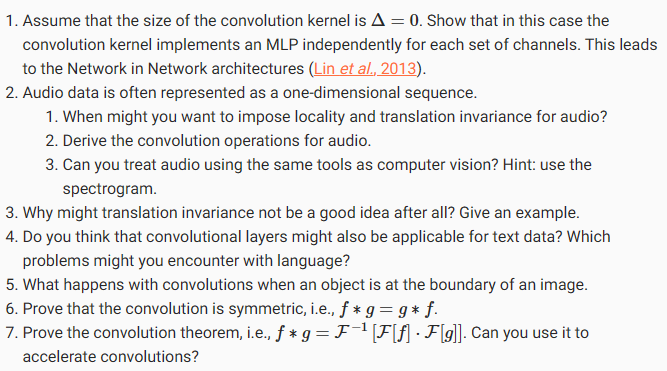
In many cases our ultimate task asks some global question about the image, e.g.,does it contain a cat?Consequently, the units of our final layer should be sensitive to the entire input. By gradually aggregating information, yielding coarser and coarser maps, we accomplish this goal of ultimately learning a global representation, while keeping all of the advantages of convolutional layers at the intermediate layers of processing. The deeper we go in the network, the larger the receptive field (relative to the input) to which each hidden node is sensitive. Reducing spatial resolution accelerates this process, since the convolution kernels cover a larger effective area.
많은 경우에 우리의 궁극적인 작업은 이미지에 대한 전반적인 질문을 합니다. (예: 고양이가 포함되어 있습니까?)결과적으로 최종 레이어의 단위는 전체 입력에 민감해야 합니다.점진적으로 정보를 집계하고 더 거칠고(coarser) 더 거친(coarser) 맵을 생성함으로써 우리는 궁극적으로 글로벌 표현(global representation)을 학습하는 동시에 중간 처리 레이어에서 컨볼루션 레이어의 모든 이점을 유지한다는 목표를 달성합니다.네트워크에 깊이 들어갈수록 각 hidden node는 민감해 지면서 수용(receptive) 필드(입력에 비해)가 커집니다.컨볼루션 커널이 더 큰 유효 영역을 다루기 때문에 공간 해상도(spatial resolution)를 줄이면 이 프로세스가 가속화됩니다.
Moreover, when detecting lower-level features, such as edges (as discussed inSection 7.2), we often want our representations to be somewhat invariant to translation. For instance, if we take the imageXwith a sharp delineation between black and white and shift the whole image by one pixel to the right, i.e.,Z[i,j]=X[i,j+1], then the output for the new imageZmight be vastly different. The edge will have shifted by one pixel. In reality, objects hardly ever occur exactly at the same place. In fact, even with a tripod and a stationary object, vibration of the camera due to the movement of the shutter might shift everything by a pixel or so (high-end cameras are loaded with special features to address this problem).
더욱 이 에지와 같은 lower-level features을 detecting할 때(섹션 7.2에서 논의됨) 우리는 종종 우리의 표현(representations)이 translation 면에서 다소 불변하기를 원합니다.예를 들어, 검은색과 흰색 사이의 뚜렷한 경계가 있는 이미지 X를 취하고 전체 이미지를 오른쪽으로 한 픽셀씩 이동하면(즉, Z[i, j] = X[i, j + 1]) 그러면 새 이미지 Z에 대한 출력은 크게 다를 수 있습니다.가장자리가 1픽셀씩 이동하게 될 겁니다.실제로는 물체가 정확히 같은 장소에 있는 경우는 거의 없습니다.사실 삼각대와 고정된 물체가 있더라도 셔터 누를때의 움직임 때문에 카메라가 약간이라도 흔들려서 모든 것들은 1픽셀이나 그 이상 움직일 수 있습니다. (고급 카메라에는 이 문제를 해결하기 위한 특수 기능이 탑재되어 있습니다).
This section introducespooling layers, which serve the dual purposes of mitigating the sensitivity of convolutional layers to location and of spatially downsampling representations.
이 섹션에서는 위치에 대한 컨볼루션 레이어의 민감도와 공간적 다운샘플링 표현의 민감도를 완화하는 이중 목적을 제공하는 풀링 레이어(pooling layers)를 소개합니다.
import torch
from torch import nn
from d2l import torch as d2l
7.5.1.Maximum Pooling and Average Pooling
Like convolutional layers,poolingoperators consist of a fixed-shape window that is slid over all regions in the input according to its stride, computing a single output for each location traversed by the fixed-shape window (sometimes known as thepooling window). However, unlike the cross-correlation computation of the inputs and kernels in the convolutional layer, the pooling layer contains no parameters (there is nokernel). Instead, pooling operators are deterministic, typically calculating either the maximum or the average value of the elements in the pooling window. These operations are calledmaximum pooling(max-poolingfor short) andaverage pooling, respectively.
컨벌루션 레이어와 마찬가지로 풀링 연산자는 보폭(stride)에 따라 입력의 모든 영역에서 미끄러지는 고정 모양 창(fixed-shape window)으로 구성되며 고정 모양 창(풀링 창이라고도 함)이 통과하는 각 위치에 대해 단일 출력을 계산합니다.그러나 컨벌루션 계층의 입력 및 커널의 상호 상관(cross-correlation) 계산과 달리 풀링 계층에는 매개 변수가 없습니다 (커널이 없음).대신 풀링 연산자는 결정적(deterministic)이며 일반적으로 풀링 창에 있는 요소의 최대값(maximum) 또는 평균값(average)을 계산합니다.이러한 작업을 각각 maximum pooling(줄여서 max-pooling) 및 평균 풀링(average pooling)이라고 합니다.
Average poolingis essentially as old as CNNs. The idea is akin to downsampling an image. Rather than just taking the value of every second (or third) pixel for the lower resolution image, we can average over adjacent pixels to obtain an image with better signal to noise ratio since we are combining the information from multiple adjacent pixels.Max-poolingwas introduced inRiesenhuber and Poggio (1999)in the context of cognitive neuroscience to describe how information aggregation might be aggregated hierarchically for the purpose of object recognition, and an earlier version in speech recognition(Yamaguchiet al., 1990). In almost all cases, max-pooling, as it is also referred to, is preferable.
평균 풀링(Average pooling)은 기본적으로 CNN만큼 오래되었습니다.아이디어는 이미지를 다운샘플링하는 것과 유사합니다.저해상도 이미지에 대해 모든 두 번째(또는 세 번째) 픽셀의 값을 취하는 대신 여러 인접 픽셀의 정보를 결합하므로 인접 픽셀에 대해 평균을 내어 더 나은 신호 대 노이즈 비율을 가진 이미지를 얻을 수 있습니다.Max-pooling은 Riesenhuber와 Poggio(1999)에서 객체 인식을 위해 정보 집계가 계층적으로 집계되는 방법을 설명하기 위해 인지 신경과학의 맥락에서 도입되었으며 음성 인식의 초기 버전(Yamaguchi et al., 1990)입니다.거의 모든 경우에 최대 풀링(max-pooling)이 선호됩니다.
In both cases, as with the cross-correlation operator, we can think of the pooling window as starting from the upper-left of the input tensor and sliding across the input tensor from left to right and top to bottom. At each location that the pooling window hits, it computes the maximum or average value of the input subtensor in the window, depending on whether max or average pooling is employed.
두 경우 모두 cross-correlation 연산자와 마찬가지로 풀링 창을 입력 텐서의 왼쪽 상단에서 시작하여 입력 텐서를 가로질러 왼쪽에서 오른쪽으로 그리고 위에서 아래로 미끄러지는 것으로 생각할 수 있습니다.풀링 윈도우가 도달하는 각 위치에서 최대 또는 평균 풀링이 사용되는지 여부에 따라 윈도우에서 입력 하위 텐서의 최대값 또는 평균값을 계산합니다.
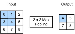
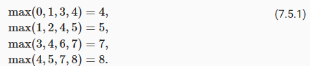
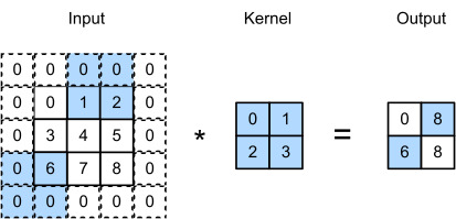
Fig. 7.5.1 Max-pooling with a pooling window shape of 2×2. The shaded portions are the first output element as well as the input tensor elements used for the output computation: max(0,1,3,4)=4.
The output tensor inFig. 7.5.1has a height of 2 and a width of 2. The four elements are derived from the maximum value in each pooling window:
그림 7.5.1의 출력 텐서는 높이가 2이고 너비가 2입니다. 4개의 요소는 각 풀링 창의 최대값에서 파생됩니다.
More generally, we can define a p×qpooling layer by aggregating over a region of said size. Returning to the problem of edge detection, we use the output of the convolutional layer as input for2×2max-pooling. Denote byXthe input of the convolutional layer input andYthe pooling layer output. Regardless of whether or not the values ofX[i,j],X[i,j+1],X[i+1,j]andX[i+1,j+1]are different, the pooling layer always outputsY[i,j]=1. That is to say, using the2×2max-pooling layer, we can still detect if the pattern recognized by the convolutional layer moves no more than one element in height or width.
보다 일반적으로, 우리는 상기 크기의 영역을 집계하여 p×q 풀링 계층을 정의할 수 있습니다.에지 감지 문제로 돌아가서 컨볼루션 레이어의 출력을 2×2 최대 풀링의 입력으로 사용합니다.X는 컨벌루션 계층 입력의 입력을 나타내고 Y는 풀링 계층 출력을 나타냅니다.X[i, j], X[i, j + 1], X[i+1, j] 및 X[i+1, j + 1]의 값이 다른지 여부에 관계없이 pooling layer는 항상Y[i, j] = 1을 출력합니다. 즉, 2×2 최대 풀링 레이어를 사용하여 컨볼루션 레이어에서 인식한 패턴이 높이 또는 너비에서 하나의 요소만 이동하는지 여전히 감지할 수 있습니다.
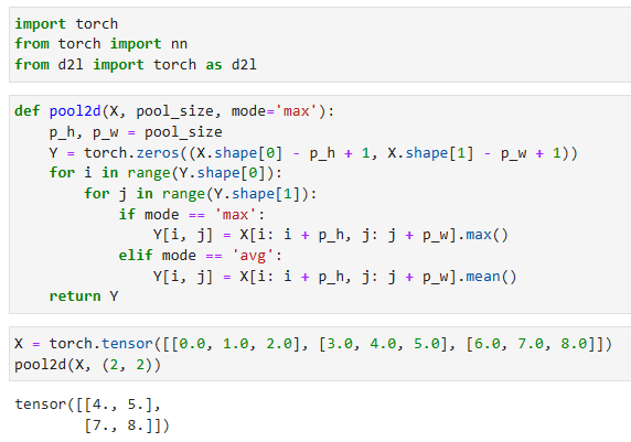
In the code below, we implement the forward propagation of the pooling layer in thepool2dfunction. This function is similar to thecorr2dfunction inSection 7.2. However, no kernel is needed, computing the output as either the maximum or the average of each region in the input.
아래 코드에서는 pool2d 함수에서 풀링 계층의 순방향 전파를 구현합니다.이 함수는 섹션 7.2의 corr2d 함수와 유사합니다.그러나 커널이 필요하지 않으며 입력에서 각 영역의 최대 또는 평균으로 출력을 계산합니다.
def pool2d(X, pool_size, mode='max'):
    p_h, p_w = pool_size
    Y = torch.zeros((X.shape[0] - p_h + 1, X.shape[1] - p_w + 1))
    for i in range(Y.shape[0]):
        for j in range(Y.shape[1]):
            if mode == 'max':
                Y[i, j] = X[i: i + p_h, j: j + p_w].max()
            elif mode == 'avg':
                Y[i, j] = X[i: i + p_h, j: j + p_w].mean()
    return Y
X는 입력 데이터로, 2차원 텐서입니다.
pool_size는 풀링 윈도우의 크기를 지정하는 튜플 (p_h, p_w)입니다.
mode는 풀링 모드를 선택하는 매개변수로, 'max' 또는 'avg'로 설정할 수 있습니다.
Y는 풀링 연산의 결과로, 입력 X의 차원을 줄여 나온 2차원 텐서입니다.
for 반복문을 사용하여 X의 각 위치에 대해 풀링 연산을 수행합니다.
mode가 'max'인 경우, 해당 위치의 풀링 윈도우에서 가장 큰 값을 선택하여 Y에 저장합니다.
mode가 'avg'인 경우, 해당 위치의 풀링 윈도우의 평균 값을 계산하여 Y에 저장합니다.
최종적으로 Y를 반환합니다.
We can construct the input tensorXinFig. 7.5.1to validate the output of the two-dimensional max-pooling layer.
그림 7.5.1에서 입력 텐서 X를 구성하여 2차원 최대 풀링 레이어의 출력을 검증할 수 있습니다.
풀링 연산은 주어진 윈도우 크기 내에서 최대값 또는 평균값을 계산하여 결과 텐서를 반환합니다.
반환된 결과 텐서는 입력 X의 크기를 줄여 2차원 텐서로 나타냅니다.
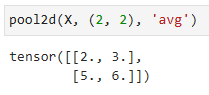
Also, we experiment with the average pooling layer.
또한 평균 풀링 계층을 실험합니다.
pool2d(X, (2, 2), 'avg')
7.5.2.Padding and Stride
As with convolutional layers, pooling layers change the output shape. And as before, we can adjust the operation to achieve a desired output shape by padding the input and adjusting the stride. We can demonstrate the use of padding and strides in pooling layers via the built-in two-dimensional max-pooling layer from the deep learning framework. We first construct an input tensorXwhose shape has four dimensions, where the number of examples (batch size) and number of channels are both 1.
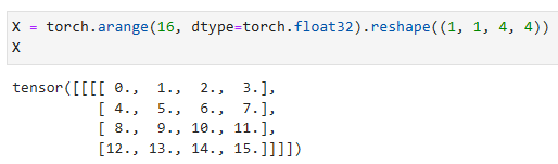
컨벌루션 레이어와 마찬가지로 풀링 레이어는 출력 형태(output shape)를 변경합니다.이전과 마찬가지로 입력을 패딩하고 보폭(stride)을 조정하여 원하는 출력 모양을 얻기 위해 작업을 조정할 수 있습니다.딥 러닝 프레임워크의 built-in two-dimensional max-pooling layer을 통해 풀링 계층에서 패딩 및 strides의 사용을 시연할 수 있습니다.먼저 모양이 4차원인 입력 텐서 X를 구성합니다. 여기서 예제 수(배치 크기)와 채널 수는 모두 1입니다.
X = torch.arange(16, dtype=torch.float32).reshape((1, 1, 4, 4))
X
torch.arange(16, dtype=torch.float32)는 0부터 15까지의 값을 가지는 1차원 텐서를 생성합니다.
.reshape((1, 1, 4, 4))는 생성된 1차원 텐서를 4x4 크기의 2차원 텐서로 변형합니다.
X는 변형된 2차원 텐서로, 형태는 (1, 1, 4, 4)입니다.
이는 배치 크기가 1이고 채널 수가 1인 4x4 크기의 이미지를 의미합니다.
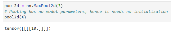
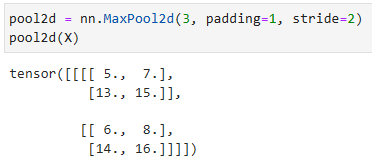
Since pooling aggregates information from an area, deep learning frameworks default to matching pooling window sizes and stride. For instance, if we use a pooling window of shape(3,3)we get a stride shape of(3,3)by default.
풀링은 한 area에서 정보를 집계하므로 딥 러닝 프레임워크는 기본적으로 일치하는 풀링 창 크기 및 보폭(stride)을 사용합니다.예를 들어 모양이 (3, 3)인 풀링 창을 사용하면 기본적으로 stride 모양이 (3, 3)이 됩니다.
pool2d = nn.MaxPool2d(3)
# Pooling has no model parameters, hence it needs no initialization
pool2d(X)
nn.MaxPool2d(3)는 3x3 크기의 Max Pooling 연산을 수행하는 풀링 레이어를 생성합니다.
풀링 레이어는 모델 파라미터가 없으므로 초기화할 필요가 없습니다.
pool2d(X)는 입력 X에 대해 Max Pooling 연산을 수행한 결과를 반환합니다.
이는 입력 이미지에서 3x3 윈도우로 최대값을 추출하여 다운샘플링한 결과입니다.
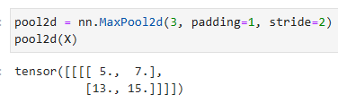
As expected, the stride and padding can be manually specified to override framework defaults if needed.
예상대로 stride과 패딩을 수동으로 특정하여 필요한 경우 프레임워크 기본값을 재정의할 수 있습니다.
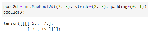
nn.MaxPool2d((2, 3), stride=(2, 3), padding=(0, 1))는 2x3 크기의 Max Pooling 연산을 수행하는 풀링 레이어를 생성합니다.
(2, 3)은 풀링 윈도우의 크기를 지정합니다. 여기서는 2x3 크기의 윈도우를 사용합니다.
stride=(2, 3)는 풀링 연산을 수행할 때 2칸씩 수평 방향으로 이동하고 3칸씩 수직 방향으로 이동하면서 다운샘플링합니다.
padding=(0, 1)은 입력에 대해 패딩을 적용하여 출력 크기를 유지합니다. 수직 방향으로만 패딩을 적용하며, 위쪽에는 패딩이 없고 아래쪽에는 1칸의 패딩을 적용합니다.
pool2d(X)는 입력 X에 대해 Max Pooling 연산을 수행한 결과를 반환합니다.
이는 입력 이미지에서 2x3 크기의 윈도우로 최대값을 추출하고, 수평과 수직 방향으로 지정된 stride만큼 이동하면서 다운샘플링한 결과입니다. 패딩을 적용하여 출력 크기를 유지합니다.
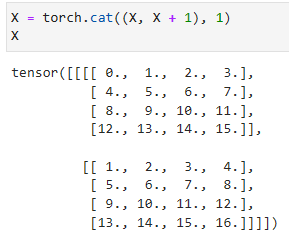
7.5.3.Multiple Channels
When processing multi-channel input data, the pooling layer pools each input channel separately, rather than summing the inputs up over channels as in a convolutional layer. This means that the number of output channels for the pooling layer is the same as the number of input channels. Below, we will concatenate tensorsXandX+1on the channel dimension to construct an input with 2 channels.
다중 채널 입력 데이터를 처리할 때 풀링 계층은 컨벌루션 계층에서와 같이 채널을 통해 입력을 합산하는 대신 각 입력 채널을 개별적으로 풀링합니다.이는 풀링 레이어의 출력 채널 수가 입력 채널 수와 같다는 것을 의미합니다.아래에서는 채널 차원에서 텐서 X와 X + 1을 연결하여 2개의 채널이 있는 입력을 구성합니다.
X = torch.cat((X, X + 1), 1)
X
torch.cat((X, X + 1), 1)은 텐서 X와 X + 1을 수평 방향(axis 1)으로 연결하는 연산입니다.
X와 X + 1은 같은 크기의 텐서이며, 수평 방향으로 연결하면 총 2개의 텐서가 결합된 결과를 반환합니다.
Pooling is an exceedingly simple operation. It does exactly what its name indicates, aggregate results over a window of values. All convolution semantics, such as strides and padding apply in the same way as they did previously. Note that pooling is indifferent to channels, i.e., it leaves the number of channels unchanged and it applies to each channel separately. Lastly, of the two popular pooling choices, max-pooling is preferable to average pooling, as it confers some degree of invariance to output. A popular choice is to pick a pooling window size of2×2to quarter the spatial resolution of output.
풀링은 매우 간단한 작업입니다.이름이 나타내는 것과 정확히 일치하며 값 창에서 결과를 집계합니다.보폭(stride) 및 패딩과 같은 모든 컨볼루션 시맨틱은 이전과 동일한 방식으로 적용됩니다.풀링은 채널과 무관합니다. 즉, 채널 수를 변경하지 않고 각 채널에 개별적으로 적용합니다.마지막으로 인기 있는 두 가지 풀링 선택 중에서 최대 풀링이 평균 풀링보다 선호되는데, 이는 출력에 어느 정도의 불변성을 부여하기 때문입니다.대중적인 선택은 2×2의 풀링 창 크기를 선택하여 출력의 공간 해상도를 4분의 1로 줄이는 것입니다.
Note that there are many more ways of reducing resolution beyond pooling. For instance, in stochastic pooling(Zeiler and Fergus, 2013)and fractional max-pooling(Graham, 2014)aggregation is combined with randomization. This can slightly improve the accuracy in some cases. Lastly, as we will see later with the attention mechanism, there are more refined ways of aggregating over outputs, e.g., by using the alignment between a query and representation vectors.
풀링 외에도 해상도를 줄이는 더 많은 방법이 있습니다.예를 들어 확률적 풀링(Zeiler and Fergus, 2013) 및 분수 최대 풀링(Graham, 2014)에서 집계는 무작위화와 결합됩니다.이것은 경우에 따라 정확도를 약간 향상시킬 수 있습니다.마지막으로 주의 메커니즘에 대해 나중에 살펴보겠지만 쿼리와 표현 벡터 사이의 정렬을 사용하여 출력을 집계하는 보다 세련된 방법이 있습니다.
While we described the multiple channels that comprise each image (e.g., color images have the standard RGB channels to indicate the amount of red, green and blue) and convolutional layers for multiple channels inSection 7.1.4, until now, we simplified all of our numerical examples by working with just a single input and a single output channel. This allowed us to think of our inputs, convolution kernels, and outputs each as two-dimensional tensors.
섹션 7.1.4에서 각 이미지를 구성하는 여러 채널(예: 컬러 이미지에는 빨강, 녹색 및 파랑의 양을 나타내는 표준 RGB 채널이 있음)과 여러 채널에 대한 컨볼루션 레이어에 대해 설명했지만 지금까지 모든 이미지를 단순화했습니다.단일 입력 및 단일 출력 채널로 작업하여 수치 예를 들어 보겠습니다.이를 통해 입력, 컨볼루션 커널 및 출력을 각각 2차원 텐서로 생각할 수 있습니다.
When we add channels into the mix, our inputs and hidden representations both become three-dimensional tensors. For example, each RGB input image has shape3×ℎ×w. We refer to this axis, with a size of 3, as thechanneldimension. The notion of channels is as old as CNNs themselves. For instance LeNet5(LeCunet al., 1995)uses them. In this section, we will take a deeper look at convolution kernels with multiple input and multiple output channels.
mix에 채널을 추가하면 입력과 hidden representations이 3차원 텐서가 됩니다.예를 들어 각 RGB 입력 이미지의 모양은 3×ℎ×w입니다.크기가 3인 이 축을 channeldimension이라고 합니다.채널의 개념은 CNN 자체만큼이나 오래되었습니다.예를 들어 LeNet5(LeCun et al., 1995)가 그것을 사용합니다.이 섹션에서는 다중 입력 및 다중 출력 채널이 있는 컨볼루션 커널에 대해 자세히 살펴보겠습니다.
import torch
from d2l import torch as d2l
7.4.1.Multiple Input Channels
When the input data contains multiple channels, we need to construct a convolution kernel with the same number of input channels as the input data, so that it can perform cross-correlation with the input data. Assuming that the number of channels for the input data is ci, the number of input channels of the convolution kernel also needs to beci. If our convolution kernel’s window shape iskℎ×kw, then whenci=1, we can think of our convolution kernel as just a two-dimensional tensor of shapekℎ×kw.
입력 데이터가 여러 채널을 포함하는 경우 입력 데이터와 상호 상관을 수행할 수 있도록 입력 데이터와 동일한 수의 입력 채널로 컨볼루션 커널을 구성해야 합니다.입력 데이터의 채널 수가 ci라고 가정하면 컨볼루션 커널의 입력 채널 수도 ci가 되어야 합니다.컨볼루션 커널의 창 모양이 kℎ×kw이면 ci=1일 때 컨볼루션 커널을 kℎ×kw 모양의 2차원 텐서로 생각할 수 있습니다.
However, whenci>1, we need a kernel that contains a tensor of shapekℎ×kwforeveryinput channel. Concatenating thesecitensors together yields a convolution kernel of shapeci×kℎ×kw. Since the input and convolution kernel each havecichannels, we can perform a cross-correlation operation on the two-dimensional tensor of the input and the two-dimensional tensor of the convolution kernel for each channel, adding theciresults together (summing over the channels) to yield a two-dimensional tensor. This is the result of a two-dimensional cross-correlation between a multi-channel input and a multi-input-channel convolution kernel.
그러나 ci>1이면 모든 입력 채널에 대해 shape kℎ×kw의 텐서를 포함하는 커널이 필요합니다.이 ci 텐서를 함께 연결하면 ci×kℎ×kw 모양의 컨볼루션 커널이 생성됩니다.입력 및 컨볼루션 커널에는 각각 ci 채널이 있으므로 각 채널에 대한 입력의 2차원 텐서와 컨볼루션 커널의 2차원 텐서에 대해 cross-correlation 연산을 수행하여 ci 결과를 함께 더할 수 있습니다(합산채널)을 사용하여 2차원 텐서를 생성합니다.이것은 다중 채널 입력과 다중 입력 채널 컨볼루션 커널 사이의 2차원 cross-correlation의 결과입니다.
Fig. 7.4.1provides an example of a two-dimensional cross-correlation with two input channels. The shaded portions are the first output element as well as the input and kernel tensor elements used for the output computation:(1×1+2×2+4×3+5×4)+(0×0+1×1+3×2+4×3)=56.
그림 7.4.1은 2개의 입력 채널이 있는 2차원 상호 상관의 예를 제공합니다.음영 부분은 출력 계산에 사용되는 입력 및 커널 텐서 요소뿐만 아니라 첫 번째 출력 요소입니다. (1×1+2×2+4×3+5×4)+(0×0+1×1+3×2+4×3)=56.
Fig. 7.4.1 Cross-correlation computation with 2 input channels.
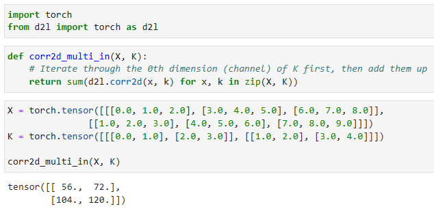
To make sure we really understand what is going on here, we can implement cross-correlation operations with multiple input channels ourselves. Notice that all we are doing is performing a cross-correlation operation per channel and then adding up the results.
여기서 무슨 일이 일어나고 있는지 확실히 이해하기 위해 여러 입력 채널을 사용하여 상호 상관 작업을 직접 구현할 수 있습니다.우리가 하는 일은 채널당 교차 상관 작업을 수행한 다음 결과를 합산하는 것뿐입니다.
def corr2d_multi_in(X, K):
    # Iterate through the 0th dimension (channel) of K first, then add them up
    return sum(d2l.corr2d(x, k) for x, k in zip(X, K))
corr2d_multi_in 함수는 다중 입력 채널에 대한 2D 크로스-코릴레이션을 수행합니다.
X는 입력 데이터를 나타내며, K는 커널을 나타냅니다.
zip(X, K)를 사용하여 X와 K를 쌍으로 묶어 순회하면서 corr2d 함수를 적용한 결과를 모두 더하여 반환합니다.
We can construct the input tensorXand the kernel tensorKcorresponding to the values inFig. 7.4.1to validate the output of the cross-correlation operation.
그림 7.4.1의 값에 해당하는 입력 텐서 X와 커널 텐서 K를 구성하여 상호 상관 연산의 출력을 검증할 수 있습니다.
X는 입력 데이터를 나타내며, shape은 (2, 3, 3)입니다. 즉, 2개의 채널을 가지며 각 채널은 3x3 크기의 2D 행렬입니다.
K는 커널을 나타내며, shape은 (2, 2, 2)입니다. 즉, 2개의 채널을 가지며 각 채널은 2x2 크기의 2D 행렬입니다.
corr2d_multi_in(X, K)를 호출하여 X와 K의 다중 입력 채널에 대한 2D 크로스-코릴레이션을 계산합니다. 결과는 (2, 2) shape을 가진 2D 텐서로 반환됩니다.
7.4.2.Multiple Output Channels
Regardless of the number of input channels, so far we always ended up with one output channel. However, as we discussed inSection 7.1.4, it turns out to be essential to have multiple channels at each layer. In the most popular neural network architectures, we actually increase the channel dimension as we go deeper in the neural network, typically downsampling to trade off spatial resolution for greaterchannel depth. Intuitively, you could think of each channel as responding to a different set of features. The reality is a bit more complicated than this. A naive interpretation would suggest that representations are learned independently per pixel or per channel. Instead, channels are optimized to be jointly useful. This means that rather than mapping a single channel to an edge detector, it may simply mean that some direction in channel space corresponds to detecting edges.
입력 채널 수에 관계없이 지금까지 우리는 항상 하나의 출력 채널로 끝났습니다.그러나 섹션 7.1.4에서 논의한 것처럼 각 계층에 여러 채널을 갖는 것이 필수적임이 밝혀졌습니다.가장 널리 사용되는 신경망 아키텍처에서 우리는 신경망이 더 깊어짐에 따라 실제로 채널 차원을 증가시키고 일반적으로 더 큰 채널 깊이를 위해 공간 해상도를 절충하기 위해 다운샘플링합니다.직관적으로 각 채널이 서로 다른 기능 집합에 응답한다고 생각할 수 있습니다.현실은 이것보다 조금 더 복잡합니다.순진한 해석은 표현이 픽셀 또는 채널별로 독립적으로 학습된다고 제안합니다.대신 채널은 공동으로 유용하도록 최적화됩니다.이는 단일 채널을 에지 검출기에 매핑하는 것이 아니라 단순히 채널 공간의 일부 방향이 에지 검출에 해당함을 의미할 수 있음을 의미합니다.
Denote by ci andcothe number of input and output channels, respectively, and letkℎandkwbe the height and width of the kernel. To get an output with multiple channels, we can create a kernel tensor of shapeci×kℎ×kwforeveryoutput channel. We concatenate them on the output channel dimension, so that the shape of the convolution kernel isco×ci×kℎ×kw. In cross-correlation operations, the result on each output channel is calculated from the convolution kernel corresponding to that output channel and takes input from all channels in the input tensor.
ci 및 co는 각각 입력 및 출력 채널의 수를 나타내고 kℎ 및 kw는 커널의 높이 및 너비입니다.여러 채널의 출력을 얻기 위해 모든 출력 채널에 대해 모양 ci×kℎ×kw의 커널 텐서를 만들 수 있습니다.컨볼루션 커널의 모양이 co×ci×kℎ×kw가 되도록 출력 채널 차원에서 이들을 연결합니다.교차 상관 연산에서 각 출력 채널의 결과는 해당 출력 채널에 해당하는 컨벌루션 커널에서 계산되며 입력 텐서의 모든 채널에서 입력을 받습니다.
We implement a cross-correlation function to calculate the output of multiple channels as shown below.
아래와 같이 여러 채널의 출력을 계산하기 위해 교차 상관 함수를 구현합니다.
def corr2d_multi_in_out(X, K):
    # Iterate through the 0th dimension of K, and each time, perform
    # cross-correlation operations with input X. All of the results are
    # stacked together
    return torch.stack([corr2d_multi_in(X, k) for k in K], 0)
X는 입력 데이터를 나타내며, shape은 (2, 3, 3)입니다. 즉, 2개의 입력 채널을 가지며 각 채널은 3x3 크기의 2D 행렬입니다.
K는 커널을 나타내며, shape은 (3, 2, 2, 2)입니다. 즉, 3개의 입력 채널과 2개의 출력 채널을 가지며 각 채널은 2x2 크기의 2D 행렬입니다.
corr2d_multi_in_out(X, K)를 호출하여 다중 입력 채널과 다중 출력 채널에 대한 2D 크로스-코릴레이션을 계산합니다. 결과는 (3, 2, 2) shape을 가진 3D 텐서로 반환됩니다.
We construct a trivial convolution kernel with 3 output channels by concatenating the kernel tensor forKwithK+1andK+2.
우리는 K에 대한 커널 텐서를 K+1 및 K+2와 연결하여 3개의 출력 채널이 있는 trivial convolution 커널을 구성합니다.
K = torch.stack((K, K + 1, K + 2), 0)
K.shape
K는 커널을 나타내는 텐서입니다.
torch.stack((K, K + 1, K + 2), 0)를 사용하여 K의 차원 0을 따라 여러 개의 커널을 쌓습니다.
결과적으로 K의 shape은 (3, 2, 2, 2)가 됩니다. 즉, 3개의 커널을 가지며 각 커널은 2개의 입력 채널과 2개의 출력 채널을 가지는 2x2 크기의 2D 행렬입니다.
Below, we perform cross-correlation operations on the input tensorXwith the kernel tensorK. Now the output contains 3 channels. The result of the first channel is consistent with the result of the previous input tensorXand the multi-input channel, single-output channel kernel.
아래에서는 입력 텐서 X와 커널 텐서 K에 대한 상호 상관 연산을 수행합니다. 이제 출력에는 3개의 채널이 포함됩니다.첫 번째 채널의 결과는 이전 입력 텐서 X 및 다중 입력 채널, 단일 출력 채널 커널의 결과와 일치합니다.
corr2d_multi_in_out(X, K)
X는 입력 데이터를 나타내는 텐서입니다.
K는 커널을 나타내는 텐서입니다.
corr2d_multi_in_out(X, K) 함수는 K의 차원 0을 따라 반복하면서 X와의 크로스-코릴레이션 연산을 수행합니다.
결과적으로 모든 결과가 스택되어 텐서로 반환됩니다. 반환된 텐서의 shape은 (3, 1, 2, 2)가 됩니다. 즉, 3개의 커널을 가지며 각 커널은 1개의 입력 채널과 2개의 출력 채널을 가지는 2x2 크기의 2D 행렬입니다.
7.4.3.1×1Convolutional Layer
At first, a1×1convolution, i.e.,kℎ=kw=1, does not seem to make much sense. After all, a convolution correlates adjacent pixels. A1×1convolution obviously does not. Nonetheless, they are popular operations that are sometimes included in the designs of complex deep networks(Linet al., 2013,Szegedyet al., 2017)Let’s see in some detail what it actually does.
처음에는 1×1 컨벌루션, 즉 kℎ=kw=1이 별 의미가 없는 것 같습니다.결국 컨볼루션은 인접한 픽셀을 연관시킵니다.1×1 컨볼루션은 분명히 그렇지 않습니다.그럼에도 불구하고 복잡한 심층 네트워크의 설계에 때때로 포함되는 인기 있는 작업입니다(Lin et al., 2013, Szegedy et al., 2017) 실제로 어떤 일을 하는지 자세히 살펴보겠습니다.
Because the minimum window is used, the1×1convolution loses the ability of larger convolutional layers to recognize patterns consisting of interactions among adjacent elements in the height and width dimensions. The only computation of the1×1convolution occurs on the channel dimension.
minimum window이 사용되기 때문에 1×1 컨볼루션은 높이와 너비 차원에서 인접한 요소 간의 상호 작용으로 구성된 패턴을 인식하는 더 큰 컨볼루션 레이어의 기능을 잃습니다.1×1 컨벌루션의 유일한 계산은 채널 차원에서 발생합니다.
Fig. 7.4.2shows the cross-correlation computation using the1×1convolution kernel with 3 input channels and 2 output channels. Note that the inputs and outputs have the same height and width. Each element in the output is derived from a linear combination of elementsat the same positionin the input image. You could think of the1×1convolutional layer as constituting a fully connected layer applied at every single pixel location to transform thecicorresponding input values intoc0output values. Because this is still a convolutional layer, the weights are tied across pixel location. Thus the1×1convolutional layer requiresco×ciweights (plus the bias). Also note that convolutional layers are typically followed by nonlinearities. This ensures that1×1convolutions cannot simply be folded into other convolutions.
그림 7.4.2는 3개의 입력 채널과 2개의 출력 채널이 있는 1×1 컨볼루션 커널을 사용한 교차 상관 계산을 보여줍니다.입력과 출력의 높이와 너비는 동일합니다.출력의 각 요소는 입력 이미지의 동일한 위치에 있는 요소의 선형 조합에서 파생됩니다.1×1 컨벌루션 레이어는 모든 단일 픽셀 위치에 적용되는 완전 연결 레이어를 구성하여 ci 해당 입력 값을 c0 출력 값으로 변환하는 것으로 생각할 수 있습니다.이것은 여전히 컨볼루션 레이어이기 때문에 가중치는 픽셀 위치 전체에 묶여 있습니다.따라서 1×1 컨벌루션 레이어에는 co×ci 가중치(바이어스 포함)가 필요합니다.또한 컨볼루션 레이어 다음에는 일반적으로 비선형성이 뒤따릅니다.이렇게 하면 1×1 컨볼루션이 단순히 다른 컨볼루션으로 접힐 수 없습니다.
Fig. 7.4.2 The cross-correlation computation uses the 1×1 convolution kernel with 3 input channels and 2 output channels. The input and output have the same height and width.
Let’s check whether this works in practice: we implement a1×1convolution using a fully connected layer. The only thing is that we need to make some adjustments to the data shape before and after the matrix multiplication.
이것이 실제로 작동하는지 확인해 보겠습니다. 완전 연결 레이어를 사용하여 1×1 컨볼루션을 구현합니다.유일한 것은 행렬 곱셈 전후에 데이터 모양을 약간 조정해야 한다는 것입니다.
def corr2d_multi_in_out_1x1(X, K):
    c_i, h, w = X.shape
    c_o = K.shape[0]
    X = X.reshape((c_i, h * w))
    K = K.reshape((c_o, c_i))
    # Matrix multiplication in the fully connected layer
    Y = torch.matmul(K, X)
    return Y.reshape((c_o, h, w))
X와 K를 형태에 맞게 재조정합니다. X는 (c_i, h * w) 형태로, K는 (c_o, c_i) 형태로 재조정됩니다.
행렬 곱셈을 통해 완전 연결 층에서의 계산을 수행합니다. Y = torch.matmul(K, X)를 통해 결과를 얻습니다.
최종적으로 Y를 (c_o, h, w) 형태로 재조정하여 반환합니다. 즉, 출력 채널 개수가 c_o이고 높이와 너비가 같은 2D 텐서를 반환합니다.
When performing1×1convolutions, the above function is equivalent to the previously implemented cross-correlation functioncorr2d_multi_in_out. Let’s check this with some sample data.
1×1 컨벌루션을 수행할 때 위의 함수는 이전에 구현된 교차 상관 함수 corr2d_multi_in_out과 동일합니다.몇 가지 샘플 데이터로 이를 확인해보자.
X는 평균 0, 표준 편차 1인 정규 분포를 따르는 3차원 텐서입니다. 크기는 (3, 3, 3)입니다.
K는 평균 0, 표준 편차 1인 정규 분포를 따르는 4차원 텐서입니다. 크기는 (2, 3, 1, 1)입니다. 이는 1x1 커널을 사용하는 다중 입력 다중 출력(conv2d_multi_in_out_1x1) 연산에 사용됩니다.
Y1은 X와 K를 사용하여 1x1 커널을 적용한 다중 입력 다중 출력(conv2d_multi_in_out_1x1) 연산의 결과입니다.
Y2는 X와 K를 사용하여 일반적인 다중 입력 다중 출력(conv2d_multi_in_out) 연산의 결과입니다.
Y1과 Y2의 차이를 절댓값으로 계산하고 그 합이 1e-6보다 작은지 확인합니다. 즉, 두 연산의 결과가 거의 동일한지 확인하는 검증(assert)입니다.
7.4.4.Discussion
Channels allow us to combine the best of both worlds: MLPs that allow for significant nonlinearities and convolutions that allow forlocalizedanalysis of features. In particular, channels allow the CNN to reason with multiple features, such as edge and shape detectors at the same time. They also offer a practical trade-off between the drastic parameter reduction arising from translation invariance and locality, and the need for expressive and diverse models in computer vision.
채널을 통해 두 세계의 장점을 결합할 수 있습니다. 중요한 비선형성을 허용하는 MLP와 기능의 국지적 분석을 허용하는 컨볼루션입니다.특히 채널을 통해 CNN은 모서리 및 모양 감지기와 같은 여러 기능을 동시에 추론할 수 있습니다.또한 변환 불변성 및 지역성으로 인해 발생하는 급격한 매개변수 감소와 컴퓨터 비전에서 표현적이고 다양한 모델에 대한 필요성 사이의 실용적인 절충안을 제공합니다.
그러나 이러한 유연성에는 대가가 따른다는 점에 유의하십시오.크기가 (ℎ×w)인 이미지가 주어지면 k×k 컨벌루션을 계산하는 비용은 O(ℎ⋅w⋅k2)입니다.ci 및 co 입력 및 출력 채널의 경우 각각 O(ℎ⋅w⋅k2⋅ci⋅co)로 증가합니다.5×5 커널과 각각 128개의 입력 및 출력 채널이 있는 256×256 픽셀 이미지의 경우 이는 530억 개가 넘는 작업에 해당합니다(곱셈과 덧셈은 별도로 계산함).나중에 우리는 ResNeXt(Xie et al., 2017)와 같은 아키텍처로 이어지는 채널별 작업이 블록 대각선이 되도록 요구함으로써 비용을 절감하는 효과적인 전략에 직면하게 될 것입니다.
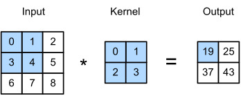
Recall the example of a convolution inFig. 7.2.1. The input had both a height and width of 3 and the convolution kernel had both a height and width of 2, yielding an output representation with dimension2×2. Assuming that the input shape isnℎ×nwand the convolution kernel shape iskℎ×kw, the output shape will be(nℎ−kℎ+1)×(nw−kw+1): we can only shift the convolution kernel so far until it runs out of pixels to apply the convolution to.
그림 7.2.1의 컨벌루션의 예를 상기하십시오.입력은 높이와 너비가 모두 3이고 컨볼루션 커널은 높이와 너비가 모두 2이므로 크기가 2×2인 출력 표현이 생성됩니다.입력 형태가 nℎ×nw이고 컨볼루션 커널 형태가 kℎ×kw라고 가정하면, 출력 형태는 (nℎ−kℎ+1)×(nw−kw+1)입니다. 컨볼루션을 적용할 픽셀이 부족해 질때 까지만 컨볼루션 커널을 이동할 수 있습니다.
In the following we will explore a number of techniques, including padding and strided convolutions, that offer more control over the size of the output. As motivation, note that since kernels generally have width and height greater than1, after applying many successive convolutions, we tend to wind up with outputs that are considerably smaller than our input. If we start with a240×240pixel image,10layers of5×5convolutions reduce the image to200×200pixels, slicing off30%of the image and with it obliterating any interesting information on the boundaries of the original image.Paddingis the most popular tool for handling this issue. In other cases, we may want to reduce the dimensionality drastically, e.g., if we find the original input resolution to be unwieldy.Strided convolutionsare a popular technique that can help in these instances.
다음에서는 패딩 및 스트라이드 컨볼루션을 포함하여 출력 크기를 더 잘 제어할 수 있는 여러 기술을 살펴보겠습니다.동기 부여로, 커널은 일반적으로 너비와 높이가 1보다 크기 때문에 많은 연속 컨볼루션을 적용한 후 입력보다 상당히 작은 출력으로 마무리되는 경향이 있습니다.240×240픽셀 이미지로 시작하면 5×5 컨볼루션의 10개 레이어가 이미지를 200×200픽셀로 축소하여 이미지의 30%를 잘라내고 원본 이미지의 경계에 대한 흥미로운 정보를 제거합니다.패딩은 이 문제를 처리하는 데 가장 널리 사용되는 도구입니다.다른 경우, 예를 들어 원래 입력 해상도가 다루기 힘든 경우와 같이 차원을 대폭 줄이고 싶을 수 있습니다.Strided convolution은 이러한 경우에 도움이 될 수 있는 인기 있는 기술입니다.
import torch
from torch import nn
7.3.1.Padding
As described above, one tricky issue when applying convolutional layers is that we tend to lose pixels on the perimeter of our image. ConsiderFig. 7.3.1that depicts the pixel utilization as a function of the convolution kernel size and the position within the image. The pixels in the corners are hardly used at all.
위에서 설명한 것처럼 컨볼루션 레이어를 적용할 때 까다로운 문제 중 하나는 이미지 주변에서 픽셀이 손실되는 경향이 있다는 것입니다.컨벌루션 커널 크기와 이미지 내 위치의 함수로 픽셀 활용도를 나타내는 그림 7.3.1을 고려하십시오.모서리의 픽셀은 거의 사용되지 않습니다.
Fig. 7.3.1 Pixel utilization for convolutions of size 1×1, 2×2, and 3×3 respectively.
Since we typically use small kernels, for any given convolution, we might only lose a few pixels, but this can add up as we apply many successive convolutional layers. One straightforward solution to this problem is to add extra pixels of filler around the boundary of our input image, thus increasing the effective size of the image. Typically, we set the values of the extra pixels to zero. InFig. 7.3.2, we pad a3×3input, increasing its size to5×5. The corresponding output then increases to a4×4matrix. The shaded portions are the first output element as well as the input and kernel tensor elements used for the output computation:0×0+0×1+0×2+0×3=0.
우리는 일반적으로 작은 커널을 사용하기 때문에 주어진 컨볼루션에 대해 몇 개의 픽셀만 손실될 수 있지만 이는 많은 연속 컨볼루션 레이어를 적용함에 따라 합산될 수 있습니다.이 문제에 대한 간단한 해결책 중 하나는 입력 이미지의 경계 주위에 필러 픽셀을 추가하여 이미지의 유효 크기를 늘리는 것입니다.일반적으로 추가 픽셀 값을 0으로 설정합니다.그림 7.3.2에서 3×3 입력을 패딩하여 크기를 5×5로 늘립니다.그러면 해당 출력이 4×4 행렬로 증가합니다.음영 부분은 첫 번째 출력 요소이자 출력 계산에 사용되는 입력 및 커널 텐서 요소입니다: 0×0+0×1+0×2+0×3=0.
Fig. 7.3.2 Two-dimensional cross-correlation with padding.
In general, if we add a total ofpℎrows of padding (roughly half on top and half on bottom) and a total ofpwcolumns of padding (roughly half on the left and half on the right), the output shape will be
일반적으로 총 pℎ 행의 패딩(대략 절반은 위쪽, 절반은 아래쪽)과 총 pw 열의 패딩(대략 왼쪽 절반, 오른쪽 절반)을 추가하면 출력 모양은 다음과 같습니다.
This means that the height and width of the output will increase bypℎandpw, respectively.
이것은 출력의 높이와 너비가 각각 pℎ와 pw만큼 증가한다는 것을 의미합니다.
In many cases, we will want to setpℎ=kℎ−1andpw=kw−1to give the input and output the same height and width. This will make it easier to predict the output shape of each layer when constructing the network. Assuming thatkℎis odd here, we will padpℎ/2rows on both sides of the height. Ifkℎis even, one possibility is to pad⌈pℎ/2⌉rows on the top of the input and⌊pℎ/2⌋rows on the bottom. We will pad both sides of the width in the same way.
대부분의 경우 입력과 출력에 동일한 높이와 너비를 제공하기 위해 pℎ=kℎ−1 및 pw=kw−1을 설정하려고 합니다.이렇게 하면 네트워크를 구성할 때 각 레이어의 출력 모양을 더 쉽게 예측할 수 있습니다.여기서 kℎ가 홀수라고 가정하면 높이 양쪽에 pℎ/2 행을 채울 것입니다.kℎ가 짝수인 경우 한 가지 가능성은 입력 상단의 ⌈pℎ/2⌉ 행과 하단의 ⌊pℎ/2⌋ 행을 채우는 것입니다.너비의 양쪽을 같은 방식으로 채웁니다.
CNNs commonly use convolution kernels with odd height and width values, such as 1, 3, 5, or 7. Choosing odd kernel sizes has the benefit that we can preserve the dimensionality while padding with the same number of rows on top and bottom, and the same number of columns on left and right.
CNN은 일반적으로 1, 3, 5 또는 7과 같은 홀수 높이 및 너비 값을 가진 컨볼루션 커널을 사용합니다. 홀수 커널 크기를 선택하면 위와 아래에 동일한 수의 행으로 패딩하면서 차원을 보존할 수 있다는 이점이 있습니다.왼쪽과 오른쪽에 같은 수의 열이 있습니다.
Moreover, this practice of using odd kernels and padding to precisely preserve dimensionality offers a clerical benefit. For any two-dimensional tensorX, when the kernel’s size is odd and the number of padding rows and columns on all sides are the same, producing an output with the same height and width as the input, we know that the outputY[i,j]is calculated by cross-correlation of the input and convolution kernel with the window centered onX[i,j].
더욱이 차원을 정확하게 보존하기 위해 홀수 커널과 패딩을 사용하는 이러한 관행은 사무적인 이점을 제공합니다.임의의 2차원 텐서 X에 대해 커널의 크기가 홀수이고 모든 면의 패딩 행과 열의 수가 동일하여 입력과 동일한 높이와 너비의 출력을 생성할 때 출력 Y[i, j]는 X[i, j]를 중심으로 하는 윈도우와 입력 및 컨벌루션 커널의 상호 상관에 의해 계산됩니다.
In the following example, we create a two-dimensional convolutional layer with a height and width of 3 and apply 1 pixel of padding on all sides. Given an input with a height and width of 8, we find that the height and width of the output is also 8.
다음 예제에서는 높이와 너비가 3인 2차원 컨볼루션 레이어를 만들고 모든 면에 1픽셀의 패딩을 적용합니다.높이와 너비가 8인 입력이 주어지면 출력의 높이와 너비도 8임을 알 수 있습니다.
# We define a helper function to calculate convolutions. It initializes the
# convolutional layer weights and performs corresponding dimensionality
# elevations and reductions on the input and output
def comp_conv2d(conv2d, X):
    # (1, 1) indicates that batch size and the number of channels are both 1
    X = X.reshape((1, 1) + X.shape)
    Y = conv2d(X)
    # Strip the first two dimensions: examples and channels
    return Y.reshape(Y.shape[2:])

# 1 row and column is padded on either side, so a total of 2 rows or columns
# are added
conv2d = nn.LazyConv2d(1, kernel_size=3, padding=1)
X = torch.rand(size=(8, 8))
comp_conv2d(conv2d, X).shape
합성곱(convolution)을 계산하기 위한 도우미 함수를 정의합니다. 이 함수는 컨볼루션 레이어 가중치를 초기화하고 입력과 출력에 대한 차원 변환을 수행합니다.
(1, 1)은 배치 크기와 채널 수가 모두 1임을 나타냅니다.
입력 X를 (1, 1) 크기로 재구성합니다. 이 때, X의 형상에 (1, 1) 차원을 추가합니다.
재구성된 입력을 사용하여 컨볼루션 레이어 conv2d를 통과시킵니다.
결과인 Y를 반환하기 전에 첫 번째와 두 번째 차원을 제거하여 형상을 조정합니다. 이는 예시와 채널 차원을 제거하는 것을 의미합니다.
conv2d는 1개의 입력 채널과 3x3 크기의 커널(kernel)을 가지는 컨볼루션 레이어를 정의합니다.
X는 8x8 크기의 랜덤한 텐서입니다.
comp_conv2d 함수를 사용하여 conv2d를 X에 적용한 결과의 형상을 확인합니다.
When the height and width of the convolution kernel are different, we can make the output and input have the same height and width by setting different padding numbers for height and width.
컨볼루션 커널의 높이와 너비가 다른 경우 높이와 너비에 다른 패딩 수를 설정하여 출력과 입력의 높이와 너비를 같게 만들 수 있습니다.
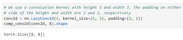
# We use a convolution kernel with height 5 and width 3. The padding on either
# side of the height and width are 2 and 1, respectively
conv2d = nn.LazyConv2d(1, kernel_size=(5, 3), padding=(2, 1))
comp_conv2d(conv2d, X).shape
높이(height)가 5이고 너비(width)가 3인 컨볼루션 커널을 사용합니다. 높이와 너비 양쪽에 대한 패딩(padding)은 각각 2와 1입니다.
conv2d는 1개의 입력 채널과 5x3 크기의 커널을 가지는 컨볼루션 레이어를 정의합니다.
앞선 설명에서 정의한 comp_conv2d 함수를 사용하여 conv2d를 X에 적용한 결과의 형상을 확인합니다.
7.3.2.Stride
When computing the cross-correlation, we start with the convolution window at the upper-left corner of the input tensor, and then slide it over all locations both down and to the right. In the previous examples, we defaulted to sliding one element at a time. However, sometimes, either for computational efficiency or because we wish to downsample, we move our window more than one element at a time, skipping the intermediate locations. This is particularly useful if the convolution kernel is large since it captures a large area of the underlying image.
상호 상관을 계산할 때 입력 텐서의 왼쪽 위 모서리에 있는 컨볼루션 창에서 시작한 다음 모든 위치를 아래로 오른쪽으로 밉니다.이전 예제에서는 기본적으로 한 번에 하나의 요소를 슬라이딩했습니다.그러나 때로는 계산 효율성을 위해 또는 다운샘플링을 원하기 때문에 중간 위치를 건너뛰고 한 번에 둘 이상의 요소를 이동합니다.이는 기본 이미지의 넓은 영역을 캡처하기 때문에 컨볼루션 커널이 큰 경우에 특히 유용합니다.
We refer to the number of rows and columns traversed per slide asstride. So far, we have used strides of 1, both for height and width. Sometimes, we may want to use a larger stride.Fig. 7.3.3shows a two-dimensional cross-correlation operation with a stride of 3 vertically and 2 horizontally. The shaded portions are the output elements as well as the input and kernel tensor elements used for the output computation:0×0+0×1+1×2+2×3=8,0×0+6×1+0×2+0×3=6. We can see that when the second element of the first column is generated, the convolution window slides down three rows. The convolution window slides two columns to the right when the second element of the first row is generated. When the convolution window continues to slide two columns to the right on the input, there is no output because the input element cannot fill the window (unless we add another column of padding).
슬라이드당 통과하는 행과 열의 수를 stride(보폭)이라고 합니다.지금까지 높이와 너비 모두에 1의 보폭(stride)을 사용했습니다.때로는 더 큰 보폭(stride)을 사용하고 싶을 수도 있습니다.그림 7.3.3은 스트라이드가 수직으로 3, 수평으로 2인 2차원 교차 상관 연산을 보여줍니다.음영 부분은 출력 요소와 출력 계산에 사용되는 입력 및 커널 텐서 요소입니다: 0×0+0×1+1×2+2×3=8, 0×0+6×1+0×2+0×3=6.첫 번째 열의 두 번째 요소가 생성되면 컨볼루션 창이 세 행 아래로 미끄러지는 것을 볼 수 있습니다.컨볼루션 창은 첫 번째 행의 두 번째 요소가 생성될 때 오른쪽으로 두 열을 슬라이드합니다.컨볼루션 창이 입력에서 오른쪽으로 두 열을 계속 슬라이드하면 입력 요소가 창을 채울 수 없기 때문에 출력이 없습니다(다른 패딩 열을 추가하지 않는 한).
Fig. 7.3.3 Cross-correlation with strides of 3 and 2 for height and width, respectively.
In general, when the stride for the height is sℎand the stride for the width issw, the output shape is
일반적으로 높이에 대한 stride를 sℎ, 너비에 대한 stride를 sw라고 하면 출력 형태는
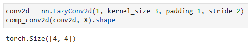
Below, we set the strides on both the height and width to 2, thus halving the input height and width.
pℎ=kℎ−1 및 pw=kw−1로 설정하면 출력 형태를 ⌊(nℎ+sℎ−1)/sℎ⌋×⌊(nw+sw−1)/sw⌋로 단순화할 수 있습니다.한 단계 더 나아가 입력 높이와 너비를 높이와 너비의 보폭으로 나눌 수 있는 경우 출력 모양은 (nℎ/sℎ)×(nw/sw)가 됩니다.
아래에서는 높이와 너비 모두에 대한 보폭을 2로 설정하여 입력 높이와 너비를 반으로 줄입니다.
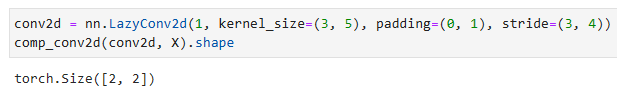
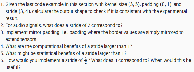
패딩(padding) 값은 (0, 1)이고 스트라이드(stride) 값은 (3, 4)인 3x5 커널을 사용하는 컨볼루션 레이어 conv2d를 정의합니다.
conv2d를 입력 데이터 X에 적용한 결과의 형상을 확인합니다.
comp_conv2d 함수를 사용하여 컨볼루션 레이어를 적용할 때의 형상 변화를 확인합니다.
7.3.3.Summary and Discussion
Padding can increase the height and width of the output. This is often used to give the output the same height and width as the input to avoid undesirable shrinkage of the output. Moreover, it ensures that all pixels are used equally frequently. Typically we pick symmetric padding on both sides of the input height and width. In this case we refer to(pℎ,pw)padding. Most commonly we setpℎ=pw, in which case we simply state that we choose paddingp.
패딩은 출력의 높이와 너비를 증가시킬 수 있습니다.이는 종종 출력이 바람직하지 않게 축소되는 것을 방지하기 위해 입력과 동일한 높이와 너비를 출력에 제공하는 데 사용됩니다.또한 모든 픽셀이 균등하게 자주 사용되도록 합니다.일반적으로 입력 높이와 너비의 양쪽에서 대칭 패딩을 선택합니다.이 경우 (pℎ,pw) 패딩을 참조합니다.가장 일반적으로 우리는 pℎ=pw를 설정합니다. 이 경우 단순히 패딩 p를 선택한다고 명시합니다.
A similar convention applies to strides. When horizontal stridesℎand vertical stride swmatch, we simply talk about strides. The stride can reduce the resolution of the output, for example reducing the height and width of the output to only1/nof the height and width of the input forn>1. By default, the padding is 0 and the stride is 1.
strides에도 유사한 규칙이 적용됩니다.수평 stride sℎ와 수직 stride sw가 일치하면 간단하게 stride s 라고 합니다.strides은 출력의 해상도를 줄일 수 있습니다. 예를 들어 출력의 높이와 너비를 n>1의 경우 입력의 높이와 너비의 1/n으로만 줄입니다.기본적으로 패딩은 0이고 스트라이드는 1입니다.
So far all padding that we discussed simply extended images with zeros. This has significant computational benefit since it is trivial to accomplish. Moreover, operators can be engineered to take advantage of this padding implicitly without the need to allocate additional memory. At the same time, it allows CNNs to encode implicit position information within an image, simply by learning where the “whitespace” is. There are many alternatives to zero-padding.Alsallakhet al.(2020)provided an extensive overview of alternatives (albeit without a clear case to use nonzero paddings unless artifacts occur).
지금까지 우리가 논의한 모든 패딩은 단순히 0으로 확장된 이미지입니다.이것은 달성하기가 쉽지 않기 때문에 계산상 상당한 이점이 있습니다.또한 연산자는 추가 메모리를 할당할 필요 없이 암시적으로 이 패딩을 활용하도록 설계할 수 있습니다.동시에 CNN은 단순히 "whitespace"이 어디에 있는지 학습함으로써 이미지 내의 암시적 위치 정보를 인코딩할 수 있습니다.제로 패딩에 대한 많은 대안이 있습니다.Alsallakhet al.(2020)은 대안에 대한 광범위한 개요를 제공했습니다(아티팩트가 발생하지 않는 한 0이 아닌 패딩을 사용하는 명확한 사례는 없지만).
Now that we understand how convolutional layers work in theory, we are ready to see how they work in practice. Building on our motivation of convolutional neural networks as efficient architectures for exploring structure in image data, we stick with images as our running example.
이제 컨볼루션 레이어가 이론적으로 어떻게 작동하는지 이해했으므로 실제로 어떻게 작동하는지 확인할 준비가 되었습니다.이미지 데이터의 구조를 탐색하기 위한 효율적인 아키텍처로서의 convolutional neural networks에 대한 motivation을Building on 하겠습니다. 우리는 이미지들을 실행 예제로 사용할 것입니다.
import torch
from torch import nn
from d2l import torch as d2l
7.2.1.The Cross-Correlation Operation
Recall that strictly speaking, convolutional layers are a misnomer, since the operations they express are more accurately described as cross-correlations. Based on our descriptions of convolutional layers inSection 7.1, in such a layer, an input tensor and a kernel tensor are combined to produce an output tensor through a cross-correlation operation.
엄밀히 말하면 컨볼루션 레이어(convolutional layers)는 잘못된 이름이라는 것을 상기하세요. 왜냐하면 그들이 표현하는 연산은 cross-correlations라고 말하는 것이 더 정확한 표현이기 때문입니다. 7.1절의 컨벌루션 레이어에 대한 설명을 기반으로 이러한 레이어에서 입력 텐서와 커널 텐서를 결합하여 cross-correlation 연산을 통해 출력 텐서를 생성합니다.
cross-correlation operation이란?
Cross-correlation is a mathematical operation that measures the similarity between two signals or sequences as they are shifted relative to each other. In the context of image processing and convolutional neural networks (CNNs), cross-correlation is commonly used for feature detection and matching.
교차 상관(Cross-correlation)은 두 신호 또는 시퀀스가 서로 이동하면서 유사성을 측정하는 수학적 연산입니다. 이미지 처리와 합성곱 신경망(CNN)의 맥락에서는 교차 상관이 특징 감지와 매칭에 일반적으로 사용됩니다.
In cross-correlation, the two signals are multiplied together at each position of the shift and then summed up. This process provides a measure of similarity or correlation between the two signals. When applied to image processing, it involves sliding a filter or kernel over an input image and computing the similarity between the filter and the corresponding image region.
교차 상관에서 두 신호는 서로의 이동 위치에서 곱해진 후 합산됩니다. 이 과정은 두 신호 간의 유사성이나 상관성을 측정하는 척도를 제공합니다. 이미지 처리에 적용할 때는 필터나 커널을 입력 이미지 위에 슬라이딩시켜 필터와 해당 이미지 영역 사이의 유사성을 계산합니다.
Cross-correlation is useful in tasks such as image recognition, object detection, and pattern matching. By comparing the similarity between a given feature or pattern and different regions of an image, cross-correlation allows for the identification of relevant features or objects.
교차 상관은 이미지 인식, 물체 감지, 패턴 매칭 등과 같은 작업에서 유용합니다. 주어진 특징이나 패턴과 이미지의 다양한 영역 간의 유사성을 비교함으로써 교차 상관은 관련 특징이나 객체를 식별하는 데 사용됩니다.
Let’s ignore channels for now and see how this works with two-dimensional data and hidden representations. InFig. 7.2.1, the input is a two-dimensional tensor with a height of 3 and width of 3. We mark the shape of the tensor as3×3or (3,3). The height and width of the kernel are both 2. The shape of thekernel window(orconvolution window) is given by the height and width of the kernel (here it is2×2).
지금은 채널을 무시하고 이것이 2차원 데이터 및 숨겨진 표현(hidden representations)에서 어떻게 작동하는지 살펴보겠습니다.그림 7.2.1에서 입력은 높이가 3이고 너비가 3인 2차원 텐서입니다. 텐서의 모양을 3×3 또는 (3, 3)으로 표시합니다.커널의 높이와 너비는 모두 2입니다. 커널 창(또는 컨볼루션 창)의 모양은 커널의 높이와 너비로 지정됩니다(여기서는 2×2).
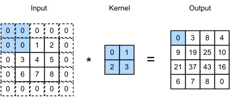
Fig. 7.2.1 Two-dimensional cross-correlation operation. The shaded portions are the first output element as well as the input and kernel tensor elements used for the output computation: 0×0+1×1+3×2+4×3=19.
In the two-dimensional cross-correlation operation, we begin with the convolution window positioned at the upper-left corner of the input tensor and slide it across the input tensor, both from left to right and top to bottom. When the convolution window slides to a certain position, the input subtensor contained in that window and the kernel tensor are multiplied elementwise and the resulting tensor is summed up yielding a single scalar value. This result gives the value of the output tensor at the corresponding location. Here, the output tensor has a height of 2 and width of 2 and the four elements are derived from the two-dimensional cross-correlation operation:
2차원 교차 상관 연산에서는 입력 텐서의 왼쪽 위 모서리에 있는 컨볼루션 창에서 시작하여 왼쪽에서 오른쪽으로 그리고 위에서 아래로 입력 텐서를 가로질러 슬라이드합니다.컨볼루션 윈도우가 특정 위치로 슬라이드되면 해당 윈도우에 포함된 입력 하위 텐서와 커널 텐서가 요소별로 곱해지고 결과 텐서가 합산되어 단일 스칼라 값이 생성됩니다.이 결과는 해당 위치에서 출력 텐서의 값을 제공합니다.여기서 출력 텐서는 높이가 2이고 너비가 2이며 4개의 요소는 2차원 교차 상관 연산에서 파생됩니다.
Note that along each axis, the output size is slightly smaller than the input size. Because the kernel has width and height greater than one, we can only properly compute the cross-correlation for locations where the kernel fits wholly within the image, the output size is given by the input size nℎ×bwminus the size of the convolution kernelkℎ×kwvia
각 축을 따라 출력 크기는 입력 크기보다 약간 작습니다. 커널의은 1보다 큰 너비와 높이가 있기 때문에 우리는 location에 대한 cross-correlation 계산만 할 수 있습니다. 출력 크기는 다음을 거쳐서 입력 크기 nℎ×nw에서 컨볼루션 커널 크기 kℎ×kw를 뺀 값입니다.
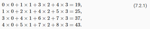
This is the case since we need enough space to “shift” the convolution kernel across the image. Later we will see how to keep the size unchanged by padding the image with zeros around its boundary so that there is enough space to shift the kernel. Next, we implement this process in thecorr2dfunction, which accepts an input tensorXand a kernel tensorKand returns an output tensorY.
이것은 이미지에서 컨볼루션 커널을 "shift"할 충분한 공간이 필요하기 때문입니다.나중에 커널을 이동할 충분한 공간이 있도록 이미지 경계 주위에 0을 채워 크기를 변경하지 않고 유지하는 방법을 살펴보겠습니다.다음으로 입력 텐서 X와 커널 텐서 K를 받아들이고 출력 텐서 Y를 반환하는 corr2d 함수에서 이 프로세스를 구현합니다.
def corr2d(X, K):  #@save
    """Compute 2D cross-correlation."""
    h, w = K.shape
    Y = torch.zeros((X.shape[0] - h + 1, X.shape[1] - w + 1))
    for i in range(Y.shape[0]):
        for j in range(Y.shape[1]):
            Y[i, j] = (X[i:i + h, j:j + w] * K).sum()
    return Y
위 코드는 2D 크로스-상관(correlation) 연산을 수행하는 함수인 corr2d를 구현한 코드입니다.
해당 코드를 한 줄씩 설명하면 다음과 같습니다:
def corr2d(X, K): : corr2d라는 함수를 정의하고, X와 K라는 두 개의 인자를 받습니다. X는 입력 데이터이고, K는 커널(필터)입니다.
h, w = K.shape : 커널의 높이 h와 너비 w를 추출합니다.
Y = torch.zeros((X.shape[0] - h + 1, X.shape[1] - w + 1)) : 출력을 저장할 Y 텐서를 생성합니다. Y의 크기는 입력 데이터와 커널의 크기에 따라 결정됩니다.
for i in range(Y.shape[0]): : Y의 행을 반복합니다.
for j in range(Y.shape[1]): : Y의 열을 반복합니다.
Y[i, j] = (X[i:i + h, j:j + w] * K).sum() : 입력 데이터 X와 커널 K 사이의 2D 크로스-상관 값을 계산하여 Y에 저장합니다. 이를 위해 입력 데이터와 커널을 요소별로 곱한 후 합을 구합니다.
return Y : 계산된 출력 텐서 Y를 반환합니다.
이 함수는 입력 데이터 X와 커널 K 사이의 2D 크로스-상관 값을 계산하여 출력하는 함수입니다. 크로스-상관은 입력 데이터와 커널 간의 유사성을 측정하는데 사용되며, 주로 이미지 처리에서 필터와 이미지의 관련성을 파악하는 데 활용됩니다.
We can construct the input tensorXand the kernel tensorKfromFig. 7.2.1to validate the output of the above implementation of the two-dimensional cross-correlation operation.
그림 7.2.1에서 입력 텐서 X와 커널 텐서 K를 구성하여 위의 2차원 교차 상관 연산의 출력을 검증할 수 있습니다.
X = torch.tensor([[0.0, 1.0, 2.0], [3.0, 4.0, 5.0], [6.0, 7.0, 8.0]])
K = torch.tensor([[0.0, 1.0], [2.0, 3.0]])
corr2d(X, K)
위 코드는 주어진 입력 데이터 X와 커널 K를 이용하여 corr2d 함수를 호출하는 코드입니다.
해당 코드를 한 줄씩 설명하면 다음과 같습니다:
X = torch.tensor([[0.0, 1.0, 2.0], [3.0, 4.0, 5.0], [6.0, 7.0, 8.0]]) : 입력 데이터인 X를 정의합니다. 이는 크기가 3x3인 텐서로, 2D 매트릭스 형태의 데이터입니다.
K = torch.tensor([[0.0, 1.0], [2.0, 3.0]]) : 커널인 K를 정의합니다. 이는 크기가 2x2인 텐서로, 2D 매트릭스 형태의 필터입니다.
corr2d(X, K) : corr2d 함수를 호출하여 입력 데이터 X와 커널 K 사이의 2D 크로스-상관 값을 계산합니다.
즉, 주어진 입력 데이터 X와 커널 K를 사용하여 corr2d 함수를 호출하고, 2D 크로스-상관 값을 계산하는 결과를 반환합니다. 이를 통해 입력 데이터와 커널 사이의 유사성을 측정하고, 컨볼루션 연산을 수행할 수 있습니다.
7.2.2.Convolutional Layers
A convolutional layer cross-correlates the input and kernel and adds a scalar bias to produce an output. The two parameters of a convolutional layer are the kernel and the scalar bias. When training models based on convolutional layers, we typically initialize the kernels randomly, just as we would with a fully connected layer.
컨볼루션 계층은 입력과 커널(혹은 필터)을 상호 연관(cross-correlates)시키고 스칼라 편향(scalar bias)을 추가하여 출력을 생성합니다.컨볼루션 레이어의 두 매개변수는 커널과 스칼라 편향((scalar bias))입니다.컨벌루션 레이어를 기반으로 모델을 교육할 때 일반적으로 완전히 연결된 레이어에서와 마찬가지로 커널을 무작위로 초기화합니다.
scalar bias란?
In the context of a convolutional layer, the scalar bias refers to a single constant value that is added to each output channel of the convolutional operation. It is an additional learnable parameter in the convolutional layer, apart from the kernel/filter weights.
합성곱 층에서의 스칼라 편향은 커널(필터)과 별개로 각 출력 채널에 더해지는 단일 상수값을 의미합니다. 합성곱 층에서 스칼라 편향은 커널 가중치 외에 추가적인 학습 가능한 매개변수입니다.
During the convolution operation, the input data is convolved with the kernel weights, and the resulting values are summed along with the scalar bias for each output channel. The scalar bias helps introduce an additional degree of freedom in the model by allowing the network to shift the output values based on the bias term.
합성곱 연산 과정에서 입력 데이터는 커널 가중치와 합성곱되고, 각 출력 채널에 대해 스칼라 편향이 더해집니다. 스칼라 편향은 신경망에게 추가적인 자유도를 부여하여 편향 항에 따라 출력 값을 조정할 수 있게 합니다.
The scalar bias allows the network to adjust the baseline or offset of the output feature maps, enabling the model to capture and represent more complex patterns and relationships in the data. It provides flexibility in modeling data with varying levels of intensity or activation.
스칼라 편향은 출력 특징 맵의 기준선 또는 오프셋을 조정할 수 있도록 합니다. 이를 통해 모델은 데이터의 다양한 강도나 활성화 수준에 따라 출력 값을 조절할 수 있게 됩니다.
In summary, the scalar bias is a single constant value added to the output channels of a convolutional layer to introduce an offset or baseline to the feature maps. It helps the model capture and represent complex patterns and relationships in the data.
요약하면, 스칼라 편향은 합성곱 층의 출력 채널에 더해지는 단일 상수값으로, 특징 맵에 기준선 또는 오프셋을 도입합니다. 이를 통해 모델은 데이터의 복잡한 패턴과 관계를 포착하고 표현할 수 있습니다.
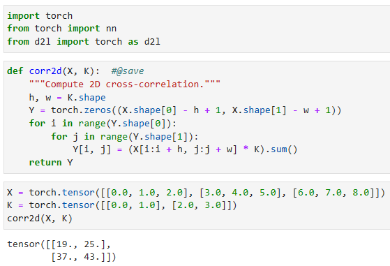
We are now ready to implement a two-dimensional convolutional layer based on thecorr2dfunction defined above. In the__init__constructor method, we declareweightandbiasas the two model parameters. The forward propagation method calls thecorr2dfunction and adds the bias.
이제 위에서 정의한 corr2d 함수를 기반으로 2차원 컨볼루션 계층을 구현할 준비가 되었습니다.__init__ 생성자 메서드에서 가중치와 편향을 두 모델 매개변수로 선언합니다.정방향 전파 방법은 corr2d 함수를 호출하고 바이어스를 추가합니다.
__init__ 메서드는 합성곱 커널 크기(kernel_size)를 입력으로 받고, 초기화 작업을 수행합니다.
self.weight는 커널 가중치를 나타내는 파라미터로 정의됩니다. torch.rand(kernel_size)를 사용하여 랜덤한 초기값으로 초기화됩니다.
self.bias는 스칼라 편향을 나타내는 파라미터로 정의됩니다. 초기값으로 0을 가집니다.
forward 메서드는 입력(x)을 받고, corr2d 함수를 사용하여 입력과 커널 가중치의 합성곱을 계산합니다. 그리고 스칼라 편향(self.bias)을 더한 결과를 반환합니다.
이 코드는 합성곱 층을 정의하고, 커널 가중치와 스칼라 편향을 포함한 학습 가능한 매개변수를 가지고 있습니다. 입력과 커널의 합성곱 결과에 편향을 더한 값이 출력으로 반환됩니다.
Inℎ×wconvolution or aℎ×wconvolution kernel, the height and width of the convolution kernel areℎandw, respectively. We also refer to a convolutional layer with aℎ×wconvolution kernel simply as aℎ×wconvolutional layer.
ℎ×w 컨볼루션 또는 ℎ×w 컨볼루션 커널에서 컨볼루션 커널의 높이와 너비는 각각 ℎ와 w입니다.또한 ℎ×w 컨볼루션 커널이 있는 컨볼루션 레이어를 단순히 ℎ×w 컨볼루션 레이어라고 합니다.
7.2.3.Object Edge Detection in Images
Let’s take a moment to parse a simple application of a convolutional layer: detecting the edge of an object in an image by finding the location of the pixel change. First, we construct an “image” of6×8pixels. The middle four columns are black (0) and the rest are white (1).
컨볼루션 레이어의 간단한 애플리케이션을 파싱하는 시간을 가져보겠습니다. 픽셀 변화의 위치를 찾아 이미지에서 객체의 가장자리를 감지합니다. 먼저 6×8 픽셀의 "이미지"를 구성합니다.가운데 4개 열은 검은색(0)이고 나머지는 흰색(1)입니다.
X = torch.ones((6, 8))
X[:, 2:6] = 0
X
X는 크기가 (6, 8)인 텐서로 초기값은 모두 1로 설정됩니다.
X[:, 2:6] = 0은 X 텐서의 모든 행(:)에서 열 인덱스 2부터 6 전까지의 범위에 해당하는 요소들을 0으로 변경합니다. 즉, 2부터 5까지의 열에 해당하는 값들을 0으로 설정합니다.
X를 출력하면 변경된 텐서가 나타납니다.
이 코드는 크기가 (6, 8)인 텐서 X를 생성한 후, 열 인덱스 2부터 5까지의 범위에 해당하는 요소들을 0으로 변경합니다. 변경된 X 텐서가 출력됩니다.
Next, we construct a kernelKwith a height of 1 and a width of 2. When we perform the cross-correlation operation with the input, if the horizontally adjacent elements are the same, the output is 0. Otherwise, the output is non-zero. Note that this kernel is special case of a finite difference operator. At location(i,j)it computesxi,j−x(i+1),j', i.e., it computes the difference between the values of horizontally adjacent pixels. This is a discrete approximation of the first derivative in the horizontal direction. After all, for a functionf(i,j)its derivative−∂if(i,j)=limϵ→0 f(i,j)−f(i+ϵ,j)/ϵ. Let’s see how this works in practice.
다음으로 높이가 1이고 너비가 2인 커널 K를 구성합니다. 입력으로 교차 상관 연산을 수행할 때 가로로 인접한 요소가 같으면 출력은 0입니다. 그렇지 않으면 출력은 0이 아닙니다.이 커널은 유한 차분 연산자(finite difference operator)의 특수한 경우입니다.위치 (i,j)에서 xi,j−x(i+1),j'를 계산합니다. 즉, 수평으로 인접한 픽셀 값 간의 차이를 계산합니다.이것은 수평 방향에서 1차 도함수의 이산 근사치(discrete approximation)입니다.결국, 함수 f(i,j)의 경우 파생물 −∂if(i,j)=limϵ→0 f(i,j)−f(i+ϵ,j)/ϵ입니다.이것이 실제로 어떻게 작동하는지 봅시다.
K = torch.tensor([[1.0, -1.0]])
K는 크기가 (1, 2)인 텐서로 초기값은 [1.0, -1.0]으로 설정됩니다.
이 코드는 크기가 (1, 2)인 텐서 K를 생성하고, 초기값으로 [1.0, -1.0]을 사용합니다.
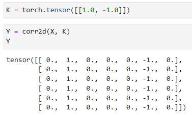
We are ready to perform the cross-correlation operation with argumentsX(our input) andK(our kernel). As you can see, we detect 1 for the edge from white to black and -1 for the edge from black to white. All other outputs take value 0.
인수 X(입력) 및 K(커널)를 사용하여 cross-correlation 연산을 수행할 준비가 되었습니다.보시다시피 흰색에서 검은색으로의 가장자리에 대해 1을 감지하고 검은색에서 흰색으로의 가장자리에 대해 -1을 감지합니다.다른 모든 출력은 값이 0입니다.
Y = corr2d(X, K)
Y
Y는 corr2d 함수에 X와 K를 입력으로 전달하여 얻은 결과입니다.
이 코드는 X와 K를 corr2d 함수에 입력으로 전달하여 얻은 결과를 Y에 할당합니다. Y는 corr2d 함수의 결과값입니다.
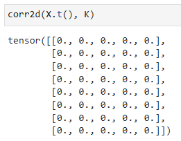
We can now apply the kernel to the transposed image. As expected, it vanishes. The kernelKonly detects vertical edges.
이제 커널을 전치된 이미지(transposed image)에 적용할 수 있습니다.예상대로 사라집니다.커널 K는 수직 에지만 감지합니다.
corr2d(X.t(), K)
corr2d 함수에 X.t()와 K를 입력으로 전달하여 호출합니다.
X.t()는 X의 전치(transpose)를 반환하는 연산입니다. 이는 X의 행과 열을 바꾼 행렬을 의미합니다.
따라서 corr2d 함수는 X의 전치된 행렬과 K를 입력으로 받아 결과를 계산합니다.
7.2.4.Learning a Kernel
Designing an edge detector by finite differences[1,-1]is neat if we know this is precisely what we are looking for. However, as we look at larger kernels, and consider successive layers of convolutions, it might be impossible to specify precisely what each filter should be doing manually.
유한 차이(finite differences) [1, -1]로 edge detector를 설계하는 것은 이것이 우리가 찾고 있는 것이 정확히 무엇인지 안다면 깔끔합니다.그러나 더 큰 커널을 살펴보고 연속적인 컨볼루션 레이어를 고려할 때 각 필터가 수동으로 수행해야 하는 작업을 정확하게 지정하는 것이 불가능할 수 있습니다.
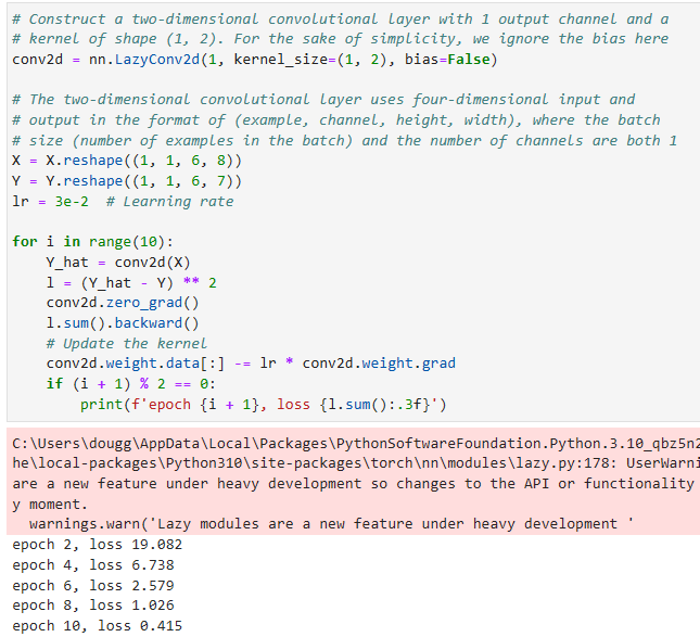
Now let’s see whether we can learn the kernel that generatedYfromXby looking at the input–output pairs only. We first construct a convolutional layer and initialize its kernel as a random tensor. Next, in each iteration, we will use the squared error to compareYwith the output of the convolutional layer. We can then calculate the gradient to update the kernel. For the sake of simplicity, in the following we use the built-in class for two-dimensional convolutional layers and ignore the bias.
이제 입력-출력 쌍만 보고 X에서 Y를 생성한 커널을 학습할 수 있는지 살펴보겠습니다.먼저 컨볼루션 레이어를 구성하고 커널을 랜덤 텐서로 초기화합니다.다음으로 각 반복에서 제곱 오차를 사용하여 Y를 컨볼루션 레이어의 출력과 비교합니다.그런 다음 기울기를 계산하여 커널을 업데이트할 수 있습니다.단순화를 위해 다음에서는 2차원 컨볼루션 레이어에 내장 클래스를 사용하고 바이어스를 무시합니다.
# Construct a two-dimensional convolutional layer with 1 output channel and a
# kernel of shape (1, 2). For the sake of simplicity, we ignore the bias here
conv2d = nn.LazyConv2d(1, kernel_size=(1, 2), bias=False)

# The two-dimensional convolutional layer uses four-dimensional input and
# output in the format of (example, channel, height, width), where the batch
# size (number of examples in the batch) and the number of channels are both 1
X = X.reshape((1, 1, 6, 8))
Y = Y.reshape((1, 1, 6, 7))
lr = 3e-2  # Learning rate

for i in range(10):
    Y_hat = conv2d(X)
    l = (Y_hat - Y) ** 2
    conv2d.zero_grad()
    l.sum().backward()
    # Update the kernel
    conv2d.weight.data[:] -= lr * conv2d.weight.grad
    if (i + 1) % 2 == 0:
        print(f'epoch {i + 1}, loss {l.sum():.3f}')
1개의 출력 채널과 (1, 2) 크기의 커널을 가지는 2D 컨볼루션 레이어(conv2d)를 생성합니다.
여기서는 편향(bias)을 고려하지 않고 설정합니다.
X와 Y를 4차원 형태로 변형하여 입력합니다. 입력과 출력은 (예제 개수, 채널 수, 높이, 너비) 형식을 따릅니다.
여기서는 배치 크기(배치에 있는 예제 수)와 채널 수가 모두 1인 형태로 설정합니다.
lr은 학습률(learning rate)로, 0.03으로 설정합니다.
for loop 문은
10번의 에폭(epoch) 동안 학습을 수행합니다.
conv2d(X)를 통해 예측값 Y_hat을 계산합니다.
손실 함수 l은 예측값과 실제값의 차이의 제곱으로 정의됩니다.
conv2d.zero_grad()를 통해 기울기를 초기화합니다.
l.sum().backward()를 통해 손실을 역전파합니다.
커널을 업데이트합니다. 업데이트는 학습률과 기울기를 이용하여 수행됩니다.
매 2번째 에폭마다 손실을 출력합니다.
Note that the error has dropped to a small value after 10 iterations. Now we will take a look at the kernel tensor we learned.
오류는 10회 반복 후 작은 값으로 떨어졌습니다.이제 우리가 배운 커널 텐서를 살펴보겠습니다.
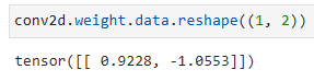
conv2d.weight.data.reshape((1, 2))
conv2d의 가중치(weight)를 (1, 2) 크기로 변형합니다.
가중치는 2D 컨볼루션 레이어에 사용되는 커널(kernel)을 나타냅니다.
(1, 2) 크기로 변형된 가중치는 1개의 출력 채널과 2개의 요소를 가지는 형태로 재구성됩니다.
Indeed, the learned kernel tensor is remarkably close to the kernel tensorKwe defined earlier.
실제로 학습된 커널 텐서는 이전에 정의한 커널 텐서 K에 매우 가깝습니다.
7.2.5.Cross-Correlation and Convolution
Recall our observation fromSection 7.1of the correspondence between the cross-correlation and convolution operations. Here let’s continue to consider two-dimensional convolutional layers. What if such layers perform strict convolution operations as defined in(7.1.6)instead of cross-correlations? In order to obtain the output of the strictconvolutionoperation, we only need to flip the two-dimensional kernel tensor both horizontally and vertically, and then perform thecross-correlationoperation with the input tensor.
교차 상관과 컨볼루션 연산 사이의 대응에 대한 섹션 7.1의 관찰을 상기하십시오.여기서 계속해서 2차원 컨볼루션 레이어를 살펴보겠습니다.이러한 레이어가 교차 상관 대신 (7.1.6)에 정의된 엄격한 컨벌루션 연산을 수행한다면 어떻게 될까요?엄격한 컨벌루션 연산의 출력을 얻기 위해서는 2차원 커널 텐서를 수평 및 수직으로 뒤집은 다음 입력 텐서와 교차 상관 연산을 수행하면 됩니다.
It is noteworthy that since kernels are learned from data in deep learning, the outputs of convolutional layers remain unaffected no matter such layers perform either the strict convolution operations or the cross-correlation operations.
커널은 딥 러닝의 데이터에서 학습되기 때문에 컨볼루션 레이어의 출력은 이러한 레이어가 strict convolution operations또는 cross-correlation operations을 수행하는 것과 상관없이 영향을 받지 않습니다.
To illustrate this, suppose that a convolutional layer performscross-correlationand learns the kernel inFig. 7.2.1, which is denoted as the matrix Khere. Assuming that other conditions remain unchanged, when this layer performs strictconvolutioninstead, the learned kernelK′will be the same asKafterK′is flipped both horizontally and vertically. That is to say, when the convolutional layer performs strictconvolutionfor the input inFig. 7.2.1andK′, the same output inFig. 7.2.1(cross-correlation of the input andK) will be obtained.
이를 설명하기 위해 합성곱 계층이 교차 상관을 수행하고 여기에서 행렬 K로 표시되는 그림 7.2.1의 커널을 학습한다고 가정합니다.다른 조건이 변하지 않는다고 가정하면, 이 레이어가 대신 엄격한 컨볼루션을 수행하면 학습된 커널 K'는 K'가 수평 및 수직으로 뒤집힌 후 K와 동일할 것입니다.즉, convolutional layer가 그림 7.2.1의 입력과 K'에 대해 엄격한 컨벌루션을 수행하면 그림 7.2.1과 동일한 출력(입력과 K의 상호 상관)이 얻어집니다.
In keeping with standard terminology with deep learning literature, we will continue to refer to the cross-correlation operation as a convolution even though, strictly-speaking, it is slightly different. Besides, we use the termelementto refer to an entry (or component) of any tensor representing a layer representation or a convolution kernel.
딥 러닝 문헌의 표준 용어에 따라 엄밀히 말하면 약간 다르지만 cross-correlationoperation을 convolution으로 계속 언급할 것입니다.게다가 element라는 용어는 layer representation 또는 convolution kernel을 나타내는 모든 텐서의 entry(또는 component)을 참조하는 데 사용됩니다.
7.2.6.Feature Map and Receptive Field
As described inSection 7.1.4, the convolutional layer output inFig. 7.2.1is sometimes called afeature map, as it can be regarded as the learned representations (features) in the spatial dimensions (e.g., width and height) to the subsequent layer. In CNNs, for any elementxof some layer, itsreceptive fieldrefers to all the elements (from all the previous layers) that may affect the calculation ofxduring the forward propagation. Note that the receptive field may be larger than the actual size of the input.
섹션 7.1.4에서 설명한 것처럼 그림 7.2.1의 컨볼루션 레이어 출력은 spatial dimensions(예: 너비 및 높이)에서 subsequent layer로 가면서 learned representations(features)으로 간주될 수 있으므로 feature map이라고도 합니다.CNN에서 일부 계층의 모든 요소 x에 대해 수용 필드는 순방향 전파 중에 x 계산에 영향을 미칠 수 있는 모든 이전 계층의 요소를 참조합니다.수용 필드는 입력의 실제 크기보다 클 수 있습니다.
Let’s continue to useFig. 7.2.1to explain the receptive field. Given the2×2convolution kernel, the receptive field of the shaded output element (of value19) is the four elements in the shaded portion of the input. Now let’s denote the2×2output as Yand consider a deeper CNN with an additional2×2convolutional layer that takesYas its input, outputting a single elementz. In this case, the receptive field ofzonYincludes all the four elements ofY, while the receptive field on the input includes all the nine input elements. Thus, when any element in a feature map needs a larger receptive field to detect input features over a broader area, we can build a deeper network.
계속해서 그림 7.2.1을 사용하여 수용 필드를 설명하겠습니다.2×2 컨볼루션 커널이 주어지면 음영 처리된 출력 요소(값 19)의 수용 필드는 입력의 음영 처리된 부분에 있는 4개의 요소입니다.이제 2×2 출력을 Y로 표시하고 Y를 입력으로 사용하여 단일 요소 z를 출력하는 추가 2×2 컨벌루션 레이어가 있는 더 깊은 CNN을 고려해 보겠습니다.이 경우 Y에 대한 z의 수용 필드는 Y의 네 가지 요소를 모두 포함하고 입력의 수용 필드는 9개의 입력 요소를 모두 포함합니다.따라서 기능 맵의 요소가 더 넓은 영역에서 입력 기능을 감지하기 위해 더 큰 수용 필드가 필요한 경우 더 깊은 네트워크를 구축할 수 있습니다.
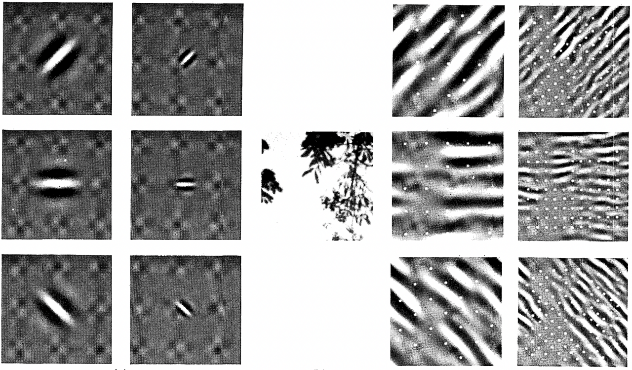
Receptive fields derive their name from neurophysiology. In a series of experiments(Hubel and Wiesel, 1959,Hubel and Wiesel, 1962,Hubel and Wiesel, 1968)on a range of animals and different stimuli, Hubel and Wiesel explored the response of what is called the visual cortex on said stimuli. By and large they found that lower levels respond to edges and related shapes. Later on,Field (1987)illustrated this effect on natural images with, what can only be called, convolutional kernels. We reprint a key figure inFig. 7.2.2to illustrate the striking similarities.
수용 분야는 신경생리학에서 이름을 따왔습니다.다양한 동물과 다양한 자극에 대한 일련의 실험(Hubel과 Wiesel, 1959, Hubel과 Wiesel, 1962, Hubel과 Wiesel, 1968)에서 Hubel과 Wiesel은 상기 자극에 대한 시각 피질이라고 불리는 것의 반응을 탐구했습니다.전반적으로 그들은 낮은 수준이 가장자리 및 관련 모양에 반응한다는 것을 발견했습니다.나중에 Field(1987)는 컨볼루션 커널이라고만 할 수 있는 자연 이미지에 대한 이 효과를 설명했습니다.놀라운 유사성을 설명하기 위해 그림 7.2.2의 핵심 수치를 다시 인쇄합니다.
Fig. 7.2.2 Figure and caption taken from Field (1987): An example of coding with six different channels. (Left) Examples of the six types of sensor associated with each channel. (Right) Convolution of the image in (Middle) with the six sensors shown in (Left). The response of the individual sensors is determined by sampling these filtered images at a distance proportional to the size of the sensor (shown with dots). This diagram shows the response of only the even symmetric sensors.
As it turns out, this relation even holds for the features computed by deeper layers of networks trained on image classification tasks, as demonstrated e.g., inKuzovkinet al.(2018). Suffice it to say, convolutions have proven to be an incredibly powerful tool for computer vision, both in biology and in code. As such, it is not surprising (in hindsight) that they heralded the recent success in deep learning.
결과적으로 Kuzovkinet al.(2018)에서 보여 주었듯 이 관계는 이미지 분류 작업에 대해 훈련된 더 깊은 네트워크 계층에서 계산된 기능에도 적용됩니다. 컨볼루션은 생물학과 코드 모두에서 컴퓨터 비전을 위한 매우 강력한 도구임이 입증되었습니다.따라서 그들이 최근 딥 러닝의 성공을 예고한 것은 (돌이켜보면) 놀라운 일이 아닙니다.
7.2.7.Summary
The core computation required for a convolutional layer is a cross-correlation operation. We saw that a simple nested for-loop is all that is required to compute its value. If we have multiple input and multiple output channels, we are performing a matrix-matrix operation between channels. As can be seen, the computation is straightforward and, most importantly, highlylocal. This affords significant hardware optimization and many recent results in computer vision are only possible due to that. After all, it means that chip designers can invest into fast computation rather than memory, when it comes to optimizing for convolutions. While this may not lead to optimal designs for other applications, it opens the door to ubiquitous and affordable computer vision.
컨볼루션 계층에 필요한 핵심 계산은 cross-correlation operation입니다.값을 계산하는 데 필요한 것은 간단한 중첩 for-loop 뿐입니다.입력 채널과 출력 채널이 여러 개인 경우 채널 간에 행렬-행렬 연산(matrix-matrix operation)을 수행합니다.여러분이 보았듯이 계산은 직관적이고 가장 중요한 것은 highly local 이라는 점입니다.이것은 상당한 하드웨어 최적화를 제공하며 컴퓨터 비전의 많은 최근 결과는 그로 인해 가능합니다.결국 이는 칩 설계자가 컨볼루션을 최적화할 때 메모리가 아닌 빠른 계산에 투자할 수 있음을 의미합니다.이것은 다른 응용 프로그램에 대한 최적의 설계로 이어지지 않을 수 있지만 유비쿼터스 및 저렴한 컴퓨터 비전의 문을 엽니다.
In terms of convolutions themselves, they can be used for many purposes such as to detect edges and lines, to blur images, or to sharpen them. Most importantly, it is not necessary that the statistician (or engineer) invents suitable filters. Instead, we can simplylearnthem from data. This replaces feature engineering heuristics by evidence-based statistics. Lastly, and quite delightfully, these filters are not just advantageous for building deep networks but they also correspond to receptive fields and feature maps in the brain. This gives us confidence that we are on the right track.
컨볼루션 자체의 측면에서 가장자리와 선을 감지하거나 이미지를 흐리게 하거나 선명하게 하는 것과 같은 다양한 목적으로 사용할 수 있습니다.가장 중요한 것은 통계학자(또는 엔지니어)가 적절한 필터를 발명할 필요가 없다는 것입니다.대신 데이터에서 간단하게 배울 수 있습니다.이는 기능 엔지니어링 휴리스틱을 증거 기반 통계로 대체합니다.마지막으로 매우 기쁘게도 이러한 필터는 심층 네트워크를 구축하는 데 유리할 뿐만 아니라 뇌의 수용 영역 및 기능 맵에 해당합니다.이것은 우리가 올바른 길을 가고 있다는 확신을 줍니다.
Image data is represented as a two-dimensional grid of pixels, be the image monochromatic or in color. Accordingly each pixel corresponds to one or multiple numerical values respectively. So far we have ignored this rich structure and treated images as vectors of numbers byflatteningthem, irrespective of the spatial relation between pixels. This deeply unsatisfying approach was necessary in order to feed the resulting one-dimensional vectors through a fully connected MLP.
이미지 데이터는 픽셀의 2차원 격자로 표현되며, 이미지는 단색이거나 컬러입니다. 따라서 각 픽셀은 각각 하나 또는 여러 개의 숫자 값에 해당합니다. 지금까지 우리는 이 풍부한 구조를 무시하고 픽셀 간의 공간적 관계에 관계없이 이미지를 평면화하여 숫자 벡터로 처리했습니다. 완전히 연결된 MLP를 통해 결과적인 1차원 벡터를 공급하려면 매우 만족스럽지 못한 이러한 접근 방식이 필요했습니다.
Because these networks are invariant to the order of the features, we could get similar results regardless of whether we preserve an order corresponding to the spatial structure of the pixels or if we permute the columns of our design matrix before fitting the MLP’s parameters. Ideally, we would leverage our prior knowledge that nearby pixels are typically related to each other, to build efficient models for learning from image data.
이러한 네트워크는 특징의 순서에 불변하기 때문에 픽셀의 공간 구조에 해당하는 순서를 유지하는지 또는 MLP의 매개변수를 맞추기 전에 디자인 행렬의 열을 순열하는지 여부에 관계없이 비슷한 결과를 얻을 수 있습니다. 이상적으로는 근처 픽셀이 일반적으로 서로 관련되어 있다는 사전 지식을 활용하여 이미지 데이터로부터 학습하기 위한 효율적인 모델을 구축합니다.
This chapter introducesconvolutional neural networks(CNNs)(LeCunet al., 1995), a powerful family of neural networks that are designed for precisely this purpose. CNN-based architectures are now ubiquitous in the field of computer vision. For instance, on the Imagnet collection(Denget al., 2009)it was only the use of convolutional neural networks, in short Convnets, that provided significant performance improvements(Krizhevskyet al., 2012).
이 장에서는 바로 이러한 목적을 위해 설계된 강력한 신경망 계열인 CNN(Convolutional Neural Network)(LeCun et al., 1995)을 소개합니다. CNN 기반 아키텍처는 이제 컴퓨터 비전 분야 어디에서나 볼 수 있습니다. 예를 들어, Imagnet 컬렉션(Deng et al., 2009)에서는 상당한 성능 향상을 제공한 것은 컨볼루션 신경망, 줄여서 Convnets의 사용뿐이었습니다(Krizhevsky et al., 2012).
Modern CNNs, as they are called colloquially, owe their design to inspirations from biology, group theory, and a healthy dose of experimental tinkering. In addition to their sample efficiency in achieving accurate models, CNNs tend to be computationally efficient, both because they require fewer parameters than fully connected architectures and because convolutions are easy to parallelize across GPU cores(Chetluret al., 2014). Consequently, practitioners often apply CNNs whenever possible, and increasingly they have emerged as credible competitors even on tasks with a one-dimensional sequence structure, such as audio(Abdel-Hamidet al., 2014), text(Kalchbrenneret al., 2014), and time series analysis(LeCunet al., 1995), where recurrent neural networks are conventionally used. Some clever adaptations of CNNs have also brought them to bear on graph-structured data(Kipf and Welling, 2016)and in recommender systems.
구어체로 불리는 현대 CNN은 생물학, 그룹 이론 및 건전한 실험적 조작에서 영감을 받아 설계되었습니다. 정확한 모델을 달성하기 위한 샘플 효율성 외에도 CNN은 완전히 연결된 아키텍처보다 적은 매개변수가 필요하고 컨볼루션이 GPU 코어 전체에서 병렬화되기 쉽기 때문에 계산적으로 효율적인 경향이 있습니다(Chetlur et al., 2014). 결과적으로 실무자들은 가능할 때마다 CNN을 적용하는 경우가 많으며 오디오(Abdel-Hamid et al., 2014), 텍스트(Kalchbrenner et al., 2014)와 같은 1차원 시퀀스 구조를 가진 작업에서도 점점 더 신뢰할 수 있는 경쟁자로 부상하고 있습니다. ), 시계열 분석(LeCun et al., 1995), 여기서는 순환 신경망이 일반적으로 사용됩니다. CNN의 일부 영리한 적응으로 인해 그래프 구조 데이터(Kipf and Welling, 2016)와 추천 시스템에도 적용되었습니다.
First, we will dive more deeply into the motivation for convolutional neural networks. This is followed by a walk through the basic operations that comprise the backbone of all convolutional networks. These include the convolutional layers themselves, nitty-gritty details including padding and stride, the pooling layers used to aggregate information across adjacent spatial regions, the use of multiple channels at each layer, and a careful discussion of the structure of modern architectures. We will conclude the chapter with a full working example of LeNet, the first convolutional network successfully deployed, long before the rise of modern deep learning. In the next chapter, we will dive into full implementations of some popular and comparatively recent CNN architectures whose designs represent most of the techniques commonly used by modern practitioners.
먼저, 컨볼루션 신경망의 동기에 대해 더 깊이 살펴보겠습니다. 그런 다음 모든 컨볼루션 네트워크의 백본을 구성하는 기본 작업을 살펴봅니다. 여기에는 컨벌루션 레이어 자체, 패딩 및 스트라이드를 포함한 핵심적인 세부 정보, 인접한 공간 영역에 걸쳐 정보를 집계하는 데 사용되는 풀링 레이어, 각 레이어에서 다중 채널 사용, 현대 아키텍처 구조에 대한 신중한 논의가 포함됩니다. 우리는 현대 딥러닝이 등장하기 오래 전에 성공적으로 배포된 최초의 컨볼루셔널 네트워크인 LeNet의 전체 작동 예제로 이 장을 마무리할 것입니다. 다음 장에서는 현대 실무자가 일반적으로 사용하는 대부분의 기술을 대표하는 디자인의 인기 있고 비교적 최근의 일부 CNN 아키텍처의 전체 구현에 대해 살펴보겠습니다.
7.1.From Fully Connected Layers to Conolutions
To this day, the models that we have discussed so far remain appropriate options when we are dealing with tabular data. By tabular, we mean that the data consist of rows corresponding to examples and columns corresponding to features. With tabular data, we might anticipate that the patterns we seek could involve interactions among the features, but we do not assume any structurea prioriconcerning how the features interact.
오늘까지 우리가 논의한 모델은 표 데이터(tabular data)를 다룰 때 적절한 옵션으로 남아 있습니다.테이블 형식(tabular data)이란 데이터가 examples에 해당하는 행과 features에 해당하는 열로 구성됨을 의미합니다.테이블 형식 데이터를 사용하면 우리가 찾는 패턴이 기능(features) 간의 상호 작용을 포함할 수 있다고 예상할 수 있지만 기능(features)이 상호 작용하는 방식과 관련하여 어떤 구조도 선험적으로 가정하지 않습니다.
Deel Learning에서 Examples 와 Features 란?
In deep learning, "examples" refer to the individual data instances or observations used for training or evaluating a model. They can be images, texts, audio clips, or any other form of input data that the model processes. Examples are typically represented as tensors or arrays of numbers to be fed into the deep learning model.
딥러닝에서 "예제(Examples)"는 모델의 학습 또는 평가를 위해 사용되는 개별 데이터 인스턴스 또는 관측치를 의미합니다. 예제는 이미지, 텍스트, 오디오 클립 또는 모델이 처리하는 다른 형태의 입력 데이터일 수 있습니다. 예제는 일반적으로 텐서나 숫자 배열로 표현되어 딥러닝 모델에 공급됩니다.
"Features" in deep learning context generally refer to the input variables or attributes that are used to represent the examples. Features are derived from the raw input data and serve as the basis for making predictions or classifications. In computer vision, for example, features may include pixel values or visual descriptors extracted from images. In natural language processing, features may be word embeddings or other text representations. The choice and quality of features can significantly impact the performance and effectiveness of a deep learning model.
"특징(Features)"은 딥러닝에서 입력 변수 또는 속성을 가리키는 용어로 사용됩니다. 특징은 원시 입력 데이터로부터 파생된 값으로, 예제를 나타내는 데 사용됩니다. 특징은 예를 들어 이미지에서 픽셀 값이나 시각적 특징 기술자로 구성될 수 있습니다. 자연어 처리에서는 단어 임베딩이나 기타 텍스트 표현이 특징으로 사용될 수 있습니다. 특징의 선택과 품질은 딥러닝 모델의 성능과 효과에 중대한 영향을 미칠 수 있습니다.
Sometimes, we truly lack knowledge to guide the construction of craftier architectures. In these cases, an MLP may be the best that we can do. However, for high-dimensional perceptual data, such structure-less networks can grow unwieldy.
때때로 우리는 더 교묘한 건축물(craftier architectures)의 건설을 안내할 지식이 정말로 부족합니다.이러한 경우 MLP가 최선일 수 있습니다.그러나 고차원 지각 데이터의 경우 이러한 구조가 없는 네트워크는 다루기 힘들게 커질 수 있습니다.
For instance, let’s return to our running example of distinguishing cats from dogs. Say that we do a thorough job in data collection, collecting an annotated dataset of one-megapixel photographs. This means that each input to the network has one million dimensions. Even an aggressive reduction to one thousand hidden dimensions would require a fully connected layer characterized by106×103=109parameters. Unless we have lots of GPUs, a talent for distributed optimization, and an extraordinary amount of patience, learning the parameters of this network may turn out to be infeasible.
예를 들어, 고양이와 개를 구별하는 예제로 돌아가 봅시다.1메가픽셀 사진의 주석이 달린 데이터 세트를 수집하는 데이터 수집 작업을 철저히 수행한다고 가정해 보겠습니다.이것은 신경망에 대한 각 입력이 백만 개의 차원을 갖는다는 것을 의미합니다.1000개의 은닉 차원으로 공격적으로 축소하더라도 106×103=109 매개변수로 특징지어지는 완전히 연결된 레이어가 필요합니다.많은 GPU, 분산 최적화 능력, 엄청난 인내심이 없다면 이 네트워크의 매개변수를 학습하는 것이 불가능할 수 있습니다.
A careful reader might object to this argument on the basis that one megapixel resolution may not be necessary. However, while we might be able to get away with one hundred thousand pixels, our hidden layer of size 1000 grossly underestimates the number of hidden units that it takes to learn good representations of images, so a practical system will still require billions of parameters. Moreover, learning a classifier by fitting so many parameters might require collecting an enormous dataset. And yet today both humans and computers are able to distinguish cats from dogs quite well, seemingly contradicting these intuitions. That is because images exhibit rich structure that can be exploited by humans and machine learning models alike. Convolutional neural networks (CNNs) are one creative way that machine learning has embraced for exploiting some of the known structure in natural images.
신중한 독자라면 1메가픽셀 해상도가 필요하지 않을 수 있다는 근거로 이 주장에 반대할 수 있습니다.그러나 10만 개의 픽셀로 벗어날 수 있지만 1000 크기의 숨겨진 레이어는 이미지의 좋은 표현을 학습하는 데 필요한 숨겨진 단위의 수를 과소 평가하므로 실제 시스템에는 여전히 수십억 개의 매개 변수가 필요합니다.또한 너무 많은 매개변수를 피팅하여 분류기를 학습하려면 막대한 데이터 세트를 수집해야 할 수 있습니다.그러나 오늘날 인간과 컴퓨터 모두 고양이와 개를 꽤 잘 구별할 수 있으며 이러한 직관과 모순되는 것처럼 보입니다.이미지는 인간과 기계 학습 모델 모두가 활용할 수 있는 풍부한 구조를 보여주기 때문입니다.CNN(컨볼루션 신경망)은 기계 학습이 자연 이미지의 알려진 구조 중 일부를 활용하기 위해 채택한 창의적인 방법 중 하나입니다.
7.1.1.Invariance (불변)
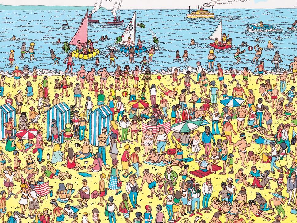
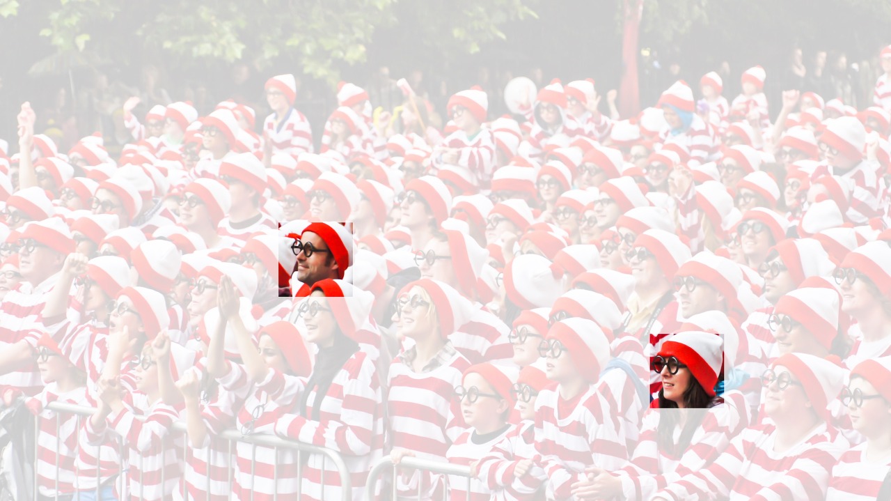
Imagine that we want to detect an object in an image. It seems reasonable that whatever method we use to recognize objects should not be overly concerned with the precise location of the object in the image. Ideally, our system should exploit this knowledge. Pigs usually do not fly and planes usually do not swim. Nonetheless, we should still recognize a pig were one to appear at the top of the image. We can draw some inspiration here from the children’s game “Where’s Waldo” (depicted inFig. 7.1.1). The game consists of a number of chaotic scenes bursting with activities. Waldo shows up somewhere in each, typically lurking in some unlikely location. The reader’s goal is to locate him. Despite his characteristic outfit, this can be surprisingly difficult, due to the large number of distractions. However,what Waldo looks likedoes not depend uponwhere Waldo is located. We could sweep the image with a Waldo detector that could assign a score to each patch, indicating the likelihood that the patch contains Waldo. In fact, many object detection and segmentation algorithms are based on this approach(Longet al., 2015). CNNs systematize this idea ofspatial invariance, exploiting it to learn useful representations with fewer parameters.
이미지를 어떤 물체인지 감지하고 싶다고 상상해 보십시오.우리가 객체를 인식하기 위해 사용하는 방법이 무엇이든 이미지에서 객체의 정확한 위치(precise location)에 지나치게 관심을 가져서는 안 된다는 것이 합리적으로 보입니다.이상적으로는 우리 시스템이 이 지식을 활용해야 합니다.돼지는 일반적으로 날지 않으며 비행기는 일반적으로 수영하지 않습니다.그럼에도 불구하고 우리는 여전히 돼지가 이미지 상단에 나타나도 돼지라는 것을 인식해야 합니다.여기서 우리는 아이들의 게임 "Waldo는 어디에 있습니까?"(그림 7.1.1에 묘사됨)에서 약간의 영감을 얻을 수 있습니다.이 게임은 활동으로 가득 찬 수많은 혼란스러운 장면으로 구성됩니다.Waldo는 각각 어딘가에 나타나며 일반적으로 가능성이 낮은 위치에 숨어 있습니다.독자의 목표는 그를 찾는 것입니다.그의 독특한 복장에도 불구하고 많은 산만함으로 인해 이것은 놀라울 정도로 어려울 수 있습니다.그러나 Waldo의 모습은 Waldo의 위치에 따라 달라지지 않습니다.각 패치에 점수를 할당할 수 있는 Waldo 탐지기로 이미지를 스윕하여 패치에 Waldo가 포함되어 있을 가능성을 나타낼 수 있습니다.실제로 많은 객체 감지 및 분할 알고리즘이 이 접근 방식을 기반으로 합니다(Long et al., 2015).CNN은 이러한 공간적 불변성(spatial invariance)에 대한 아이디어를 체계화하여 이를 활용하여 더 적은 매개변수로 유용한 표현을 학습합니다.
Fig. 7.1.1 An image of the “Where’s Waldo” game.
We can now make these intuitions more concrete by enumerating a few desiderata to guide our design of a neural network architecture suitable for computer vision:
이제 우리는 컴퓨터 비전에 적합한 신경망 아키텍처 설계를 안내하기 위해 몇 가지 필요한 사항을 열거함으로써 이러한 직관을 보다 구체적으로 만들 수 있습니다.
In the earliest layers, our network should respond similarly to the same patch, regardless of where it appears in the image. This principle is calledtranslation invariance(ortranslation equivariance). 초기 레이어에서 네트워크는 이미지의 어디에 표시되는지에 관계없이 동일한 패치(patch)에 유사하게 응답해야 합니다.이 원칙을 translation invariance (또는 translation equivariance-)이라고 합니다.
The earliest layers of the network should focus on local regions, without regard for the contents of the image in distant regions. This is thelocalityprinciple. Eventually, these local representations can be aggregated to make predictions at the whole image level. 네트워크의 가장 초기 계층은 먼 지역에 있는 이미지의 내용을 고려하지 않고 로컬 지역에 초점을 맞춰야 합니다.이것이 지역성의 원칙(localityprinciple)입니다.결국 이러한 로컬 representations을 집계하여 전체 이미지 수준에서 예측할 수 있습니다.
As we proceed, deeper layers should be able to capture longer-range features of the image, in a way similar to higher level vision in nature. 진행함에 따라 더 깊은 레이어는 자연의 더 높은 수준의 비전과 유사한 방식으로 이미지의 장거리 기능(longer-range features)을 캡처할 수 있어야 합니다.
Let’s see how this translates into mathematics.
이것이 어떻게 수학으로 변환되는지 봅시다.
7.1.2.Constraining the MLP
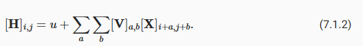
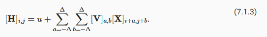
To start off, we can consider an MLP with two-dimensional images Xas inputs and their immediate hidden representationsHsimilarly represented as matrices (they are two-dimensional tensors in code), where bothXandHhave the same shape. Let that sink in. We now conceive of not only the inputs but also the hidden representations as possessing spatial structure.
우선, 2차원 이미지 X를 입력으로 사용하는 MLP를 생각해 볼 수 있습니다. 그들의 immediate hidden representationsH는 matrices(그들은 코드에서 2차원 텐서입니다.)로서 두 X와 H가 같은 모양을 갖기 때문에 유사하게 표현됩니다. 좀 더 깊이 들어 갑시다. 우리는 이제 입력뿐만 아니라 hidden representations도 spatial structure를 가지고 있다고 생각합니다.
Let[X]i,jand[H]i,jdenote the pixel at location(i,j)in the input image and hidden representation, respectively. Consequently, to have each of the hidden units receive input from each of the input pixels, we would switch from using weight matrices (as we did previously in MLPs) to representing our parameters as fourth-order weight tensorsW. Suppose thatUcontains biases, we could formally express the fully connected layer as
[X]i,j 및 [H]i,j는 각각 입력 이미지 및 hidden representation의 location(i,j)에 있는 픽셀을 나타냅니다.결과적으로 각각의 은닉 유닛(hidden units)이 각 입력 픽셀로부터 입력을 받도록 하려면 가중치 행렬-weight matrices-(이전에 MLP에서 했던 것처럼)을 사용하는 것에서 매개변수를 4차 가중치 텐서 W(fourth-order weight tensorsW)로 나타내는 것으로 전환해야 합니다. U가 편향을 포함한다고 가정합니다. 우리는 fully connected layer를 공식적으로 다음과 같이 표현할 수 있습니다.
The switch fromWtoVis entirely cosmetic for now since there is a one-to-one correspondence between coefficients in both fourth-order tensors. We simply re-index the subscripts(k,l)such thatk=i+aandl=j+b. In other words, we set[V]i,j,a,b=[W]i,j,i+a,j+b. The indicesaandbrun over both positive and negative offsets, covering the entire image. For any given location (i,j) in the hidden representation[H]i,j, we compute its value by summing over pixels inx, centered around(i,j)and weighted by[V]i,j,a,b. Before we carry on, let’s consider the total number of parameters required for asinglelayer in this parametrization: a1000×1000image (1 megapixel) is mapped to a1000×1000hidden representation. This requires1012parameters, far beyond what computers currently can handle.
W에서 V로의 전환은 두 4차 텐서(fourth-order tensors)의 계수(coefficients) 사이에 일대일 대응이 있기 때문에 현재로서는 완전히 외관상(cosmetic)입니다.우리는 단순히 k=i+a 및 l=j+b와 같이 subscripts (k,l)를 다시 인덱싱합니다.즉, [V]i,j,a,b=[W]i,j,i+a,j+b로 설정합니다.인덱스 a와 b는 양수 오프셋과 음수 오프셋 모두에서 실행되어 전체 이미지를 덮습니다.숨겨진 표현(hidden representation) [H]i,j의 주어진 위치(location)(i, j)에 대해 x의 픽셀을 합산하여 값을 계산하고 (i,j)를 중심으로 [V]i,j,a,b에 의해 가중치를 적용합니다.계속하기 전에 이 매개변수화에서 단일 레이어에 필요한 총 매개변수 수를 고려해 보겠습니다. 1000×1000 이미지(1메가픽셀)는 1000×1000 숨겨진 표현에 매핑(hidden representation)됩니다.여기에는 컴퓨터가 현재 처리할 수 있는 것보다 훨씬 많은 1012개의 매개변수가 필요합니다.
hidden representation 이란?
Hidden representation refers to the intermediate or hidden layers of a neural network where the input data is transformed and processed before reaching the final output layer. It is a set of internal representations or features that capture relevant information about the input data.
'Hidden representation'은 신경망의 중간 또는 숨겨진 레이어로, 입력 데이터가 최종 출력 레이어에 도달하기 전에 변환되고 처리되는 부분을 의미합니다. 이는 입력 데이터에 대한 관련 정보를 포착하는 내부 표현이나 피처들의 집합입니다.
In a neural network, the hidden layers perform computations on the input data using a combination of weights, biases, and activation functions. Each hidden layer progressively extracts higher-level features or abstractions from the raw input data. These hidden representations are not directly observable or interpretable by humans but contain important information that helps the network make accurate predictions or classifications.
신경망에서는 숨겨진 레이어들이 가중치, 편향, 활성화 함수의 조합을 사용하여 입력 데이터에 대해 계산을 수행합니다. 각 숨겨진 레이어는 원시 입력 데이터로부터 점차적으로 고수준의 피처나 추상화를 추출합니다. 이러한 숨겨진 표현은 직접적으로 사람들에게 관측 가능하거나 해석 가능한 것은 아니지만, 네트워크가 정확한 예측이나 분류를 수행하는 데 도움이 되는 중요한 정보를 포함합니다.
The purpose of hidden representations is to capture meaningful and relevant patterns in the data that are useful for the specific task the neural network is designed to solve. By learning these representations through the training process, neural networks can automatically discover complex relationships and hierarchical structures in the data, leading to improved performance and generalization.
숨겨진 표현의 목적은 신경망이 해결하려는 특정 작업에 유용한 데이터의 의미 있는 패턴을 포착하는 것입니다. 훈련 과정을 통해 이러한 표현을 학습함으로써 신경망은 데이터에서 복잡한 관계와 계층 구조를 자동으로 발견할 수 있습니다. 이를 통해 성능과 일반화 능력이 향상됩니다.
Overall, hidden representations play a crucial role in deep learning as they enable the network to learn and represent data in a more compact and expressive form, facilitating effective information processing and learning.
전반적으로, 숨겨진 표현은 딥 러닝에서 중요한 역할을 하며, 네트워크가 데이터를 더 간결하고 표현력이 풍부한 형태로 학습하고 표현할 수 있도록 돕습니다. 이는 효과적인 정보 처리와 학습을 가능하게 하며, 네트워크의 성능 향상에 기여합니다.
7.1.2.1.Translation Invariance
Now let’s invoke the first principle established above: translation invariance(Zhang and others, 1988). This implies that a shift in the inputXshould simply lead to a shift in the hidden representationH. This is only possible ifVandUdo not actually depend on(i,j). As such, we have[V]i,j,a,b=[V]a,bandUis a constant, sayu. As a result, we can simplify the definition forH:
이제 위에서 확립한 첫 번째 원칙인 변환 불변성(translation invariance)을 적용해 보겠습니다(Zhang and others, 1988).이는 입력 X의 이동이 단순히 숨겨진 표현(hidden representation) H의 이동으로 이어져야 함을 의미합니다. 이것은 V와 U가 실제로 (i,j)에 의존하지 않는 경우에만 가능합니다.따라서 [V]i,j,a,b=[V]a,b이고 U는 상수입니다.결과적으로 H에 대한 정의를 단순화할 수 있습니다.
This is aconvolution! We are effectively weighting pixels at(i+a,j+b)in the vicinity of location(i,j)with coefficients[V]a,bto obtain the value[H]i,j. Note that[V]a,bneeds many fewer coefficients than[V]i,j,a,bsince it no longer depends on the location within the image. Consequently, the number of parameters required is no longer1012but a much more reasonable4⋅106: we still have the dependency ona,b∈(−1000,1000). In short, we have made significant progress. Time-delay neural networks (TDNNs) are some of the first examples to exploit this idea(Waibelet al., 1989).
이것은 convolution입니다!값 [H]i,j를 얻기 위해 계수(coefficients)a,b를 사용하여 위치 (i,j) 부근의 (i+a,j+b)에 있는 픽셀에 효과적으로 가중치를 부여합니다.[V]a,b는 더 이상 이미지 내의 위치에 의존하지 않기 때문에 [V]i,j,a,b보다 훨씬 적은 계수가 필요합니다.결과적으로 필요한 매개변수의 수는 더 이상 1012가 아니라 훨씬 더 합리적인 4⋅106입니다. 여전히 a,b∈(−1000,1000)에 대한 종속성이 있습니다.요컨대, 우리는 상당한 진전을 이루었습니다.시간 지연 신경망-Time-delay neural networks-(TDNN)은 이 아이디어를 활용한 첫 번째 사례 중 일부입니다(Waibel et al., 1989).
Translation Invariance란?
Translation invariance in convolutional neural networks (CNNs) refers to the property of CNNs to recognize patterns or features in an input image regardless of their position or location within the image. It means that if an object or feature is present in different parts of the image, the CNN will be able to detect and identify it regardless of its specific location.
합성곱 신경망(Convolutional Neural Networks, CNNs)의 변환 불변성(Translation Invariance)은 CNN이 입력 이미지 내에서 위치나 위치에 관계없이 패턴이나 특징을 인식하는 성질을 의미합니다. 이는 이미지 내에 객체나 특징이 다른 위치에 존재할 경우, CNN이 그것을 인식하고 식별할 수 있다는 것을 의미합니다.
CNNs achieve translation invariance through the use of convolutional layers and pooling layers. Convolutional layers apply filters or kernels to scan the entire input image, detecting local patterns or features. These filters are shared across the entire image, allowing the CNN to learn and recognize the same patterns regardless of their position. Pooling layers further enhance translation invariance by downsampling the feature maps, reducing the spatial dimensions while retaining important features.
CNN은 합성곱 계층(Convolutional Layers)과 풀링 계층(Pooling Layers)을 사용하여 변환 불변성을 달성합니다. 합성곱 계층은 필터 또는 커널을 사용하여 전체 입력 이미지를 스캔하며 지역적인 패턴이나 특징을 감지합니다. 이러한 필터는 이미지 전체에 걸쳐 공유되며, CNN은 위치에 상관없이 동일한 패턴을 학습하고 인식할 수 있습니다. 풀링 계층은 특징 맵을 다운샘플링하여 공간적인 차원을 줄이고 중요한 특징을 유지함으로써 변환 불변성을 강화합니다.
This translation invariance property makes CNNs well-suited for tasks such as image classification, object detection, and image segmentation, where the position or location of objects or features within an image may vary. It enables CNNs to effectively learn and generalize spatial patterns across different parts of an image.
이러한 변환 불변성은 CNN을 이미지 분류, 객체 탐지, 이미지 세그멘테이션과 같은 작업에 적합하게 만듭니다. 이미지 내 객체나 특징의 위치가 다양하게 변할 수 있는 경우에도 CNN은 효과적으로 공간 패턴을 학습하고 일반화할 수 있게 됩니다.
7.1.2.2.Locality
Now let’s invoke the second principle: locality. As motivated above, we believe that we should not have to look very far away from location(i,j)in order to glean relevant information to assess what is going on at[H]i,j. This means that outside some range|a|>Δor|b|>Δ, we should set[V]a,b=0. Equivalently, we can rewrite[H]i,jas
이제 두 번째 원칙인 지역성을 적용해 보겠습니다.위에서 동기부여된 바와 같이, 우리는 [H]i,j에서 무슨 일이 일어나고 있는지 평가하기 위해 관련 정보를 수집하기 위해 위치 (i,j)에서 아주 멀리 볼 필요가 없다고 믿습니다.이는 어떤 범위 |a|>Δ 또는 |b|>Δ를 벗어나면 [V]a,b=0으로 설정해야 함을 의미합니다.마찬가지로 [H]i,j를 다음과 같이 다시 쓸 수 있습니다.
This reduces the number of parameters from4⋅106to4Δ2, whereΔis typically smaller than10. As such, we reduced the number of parameters by another 4 orders of magnitude. Note that(7.1.3), in a nutshell, is what is called aconvolutional layer.Convolutional neural networks(CNNs) are a special family of neural networks that contain convolutional layers. In the deep learning research community,Vis referred to as aconvolution kernel, afilter, or simply the layer’sweightsthat are learnable parameters.
이렇게 하면 매개변수 수가 4⋅106에서 4Δ2로 줄어듭니다. 여기서 Δ는 일반적으로 10보다 작습니다. 따라서 매개변수 수를 4배 더 줄였습니다.간단히 말해서 (7.1.3)은 컨볼루션 레이어(convolutional layer)라고 합니다.컨볼루션 신경망-Convolutional neural networks-(CNN)은 컨볼루션 레이어(convolutional layer)를 포함하는 neural networks의 special family입니다.딥 러닝 연구 커뮤니티에서 V는 컨볼루션 커널(convolution kernel), 필터 또는 단순히 학습 가능한 매개변수인 레이어의 가중치(weights)라고 합니다.
While previously, we might have required billions of parameters to represent just a single layer in an image-processing network, we now typically need just a few hundred, without altering the dimensionality of either the inputs or the hidden representations. The price paid for this drastic reduction in parameters is that our features are now translation invariant and that our layer can only incorporate local information, when determining the value of each hidden activation. All learning depends on imposing inductive bias. When that bias agrees with reality, we get sample-efficient models that generalize well to unseen data. But of course, if those biases do not agree with reality, e.g., if images turned out not to be translation invariant, our models might struggle even to fit our training data.
이전에는 이미지 처리 네트워크의 단일 레이어를 나타내기 위해 수십억 개의 매개변수가 필요했지만 이제는 입력 또는 숨겨진 표현(hidden representations)의 차원을 변경하지 않고 일반적으로 수백 개만 필요합니다.이러한 매개 변수의 급격한 감소에 대해 지불한 대가는 우리의 기능이 이제 변환 불변(translation invariant)이고 레이어가 각 숨겨진 활성화 값을 결정할 때 로컬 정보만 통합할 수 있다는 것입니다.모든 학습은 귀납적 편향(inductive bias)을 부과하는 데 달려 있습니다.그 편견(bias)이 현실과 일치할 때 우리는 보이지 않는 데이터에 잘 일반화되는 sample-efficient models을 얻습니다.그러나 물론 이러한 편향(bias)이 현실과 일치하지 않는 경우(예: 이미지가 변환 불변(translation invariant)이 아닌 것으로 판명된 경우) 모델이 훈련 데이터에 맞추는 데 어려움을 겪을 수 있습니다.
This dramatic reduction in parameters brings us to our last desideratum, namely that deeper layers should represent larger and more complex aspects of an image. This can be achieved by interleaving nonlinearities and convolutional layers repeatedly.
이러한 매개변수의 극적인 감소는 마지막 요구사항, 즉 더 깊은 레이어가 이미지의 더 크고 더 복잡한 측면을 나타내야 한다는 점을 의미합니다.이는 비선형성과 컨벌루션 레이어를 반복적으로 interleaving하여 달성할 수 있습니다.
7.1.3.Convolutions
Let’s briefly review why(7.1.3)is called a convolution. In mathematics, theconvolutionbetween two functions(Rudin, 1973), sayf,g:ℝd→ℝis defined as
(7.1.3)이 컨볼루션이라고 불리는 이유를 간단히 살펴보겠습니다.수학에서 f,g:ℝd→ℝ와 같이 두 함수 간의 컨볼루션(Rudin, 1973)은 다음과 같이 정의됩니다.
That is, we measure the overlap betweenfandgwhen one function is “flipped” and shifted byx. Whenever we have discrete objects, the integral turns into a sum. For instance, for vectors from the set of square summable infinite dimensional vectors with index running overℤwe obtain the following definition:
즉, 하나의 함수가 "플립"되고 x만큼 이동될 때 f와 g 사이의 중첩을 측정합니다.이산 객체(discrete objects)가 있을 때마다 적분(integral)은 합계로 바뀝니다.예를 들어, 인덱스가 ℤ 이상인 제곱 합산 가능한 무한 차원 벡터 세트의 벡터에 대해 다음 정의를 얻습니다.
For two-dimensional tensors, we have a corresponding sum with indices(a,b)forfand(i−a,j−b)forg, respectively:
2차원 텐서의 경우 각각 f에 대한 인덱스 (a,b)와 g에 대한 (i-a,j-b)의 해당 합계가 있습니다.
This looks similar to(7.1.3), with one major difference. Rather than using(i+a,j+b), we are using the difference instead. Note, though, that this distinction is mostly cosmetic since we can always match the notation between(7.1.3)and(7.1.6). Our original definition in(7.1.3)more properly describes across-correlation. We will come back to this in the following section.
이것은 (7.1.3)과 비슷해 보이지만 한 가지 중요한 차이점이 있습니다.(i+a,j+b)를 사용하는 대신 차이점을 대신 사용합니다.하지만 (7.1.3)과 (7.1.6) 사이의 표기법을 항상 일치시킬 수 있기 때문에 이 구별은 대부분 외형적(cosmetic)입니다.(7.1.3)의 원래 정의는 교차 상관(cross-correlation)을 더 적절하게 설명합니다.이에 대해서는 다음 섹션에서 다시 설명하겠습니다.
7.1.4.Channels
Returning to our Waldo detector, let’s see what this looks like. The convolutional layer picks windows of a given size and weighs intensities according to the filterV, as demonstrated inFig. 7.1.2. We might aim to learn a model so that wherever the “waldoness” is highest, we should find a peak in the hidden layer representations.
Waldo 감지기로 돌아가서 이것이 어떻게 보이는지 봅시다.컨볼루션 레이어는 주어진 크기의 창을 선택하고 그림 7.1.2에서 보여지는 것처럼 필터 V에 따라 강도를 가중합니다."waldoness"가 가장 높은 곳에서 숨겨진 레이어 표현에서 최고점을 찾도록 모델 학습을 목표로 할 수 있습니다.
Fig. 7.1.2 Detect Waldo.
There is just one problem with this approach. So far, we blissfully ignored that images consist of 3 channels: red, green, and blue. In sum, images are not two-dimensional objects but rather third-order tensors, characterized by a height, width, and channel, e.g., with shape1024×1024×3pixels. While the first two of these axes concern spatial relationships, the third can be regarded as assigning a multidimensional representation to each pixel location. We thus indexXas[X]i,j,k. The convolutional filter has to adapt accordingly. Instead of[V]a,b, we now have[V]a,b,c.
이 접근 방식에는 한 가지 문제가 있습니다.지금까지 우리는 이미지가 빨강, 초록, 파랑의 3개 채널로 구성되어 있다는 사실을 다행스럽게도 무시했습니다.요컨대 이미지는 2차원 객체가 아니라 높이, 너비 및 채널(예: 1024×1024×3 픽셀 모양)로 특징지어지는 3차 텐서입니다.이러한 축 중 처음 두 개는 공간 관계(spatial relationships)와 관련이 있지만 세 번째 축은 각 픽셀 위치에 다차원 표현을 할당하는 것으로 간주할 수 있습니다.따라서 X를 [X]i,j,k로 인덱싱합니다.컨벌루션 필터는 그에 따라 adapt해야 합니다.[V]a,b 대신 이제 [V]a,b,c가 있습니다.
Moreover, just as our input consists of a third-order tensor, it turns out to be a good idea to similarly formulate our hidden representations as third-order tensorsH. In other words, rather than just having a single hidden representation corresponding to each spatial location, we want an entire vector of hidden representations corresponding to each spatial location. We could think of the hidden representations as comprising a number of two-dimensional grids stacked on top of each other. As in the inputs, these are sometimes calledchannels. They are also sometimes calledfeature maps, as each provides a spatialized set of learned features to the subsequent layer. Intuitively, you might imagine that at lower layers that are closer to inputs, some channels could become specialized to recognize edges while others could recognize textures.
또한 입력이 3차 텐서로 구성되는 것처럼 숨겨진 표현을 3차 텐서 H로 유사하게 공식화하는 것이 좋습니다.즉, 각 공간 위치에 해당하는 단일 숨겨진 표현(hidden representation)이 아니라 각 공간 위치에 해당하는 숨겨진 표현(hidden representation)의 전체 벡터가 필요합니다.숨겨진 표현(hidden representation)은 서로 위에 쌓인 여러 개의 2차원 그리드로 구성되어 있다고 생각할 수 있습니다.입력과 마찬가지로 이를 채널이라고도 합니다.각각은 학습된 기능의 공간화된 세트를 후속 계층에 제공하기 때문에 기능 맵이라고도 합니다.직관적으로 입력에 더 가까운 하위 레이어에서 일부 채널은 가장자리를 인식하도록 특수화되고 다른 채널은 텍스처를 인식할 수 있다고 상상할 수 있습니다.
To support multiple channels in both inputs (X) and hidden representations (H), we can add a fourth coordinate toV:[V]a,b,c,d. Putting everything together we have:
입력(X)과 숨겨진 표현(H) 모두에서 다중 채널을 지원하기 위해 V에 네 번째 좌표인 [V]a,b,c,d를 추가할 수 있습니다.모든 것을 종합하면 다음과 같습니다.
wheredindexes the output channels in the hidden representationsH. The subsequent convolutional layer will go on to take a third-order tensor,H, as input. Being more general,(7.1.7)is the definition of a convolutional layer for multiple channels, whereVis a kernel or filter of the layer.
여기서 d는 숨겨진 표현 H의 출력 채널을 인덱싱합니다. 후속 컨볼루션 레이어는 계속해서 3차 텐서 H를 입력으로 사용합니다.보다 일반적으로 (7.1.7)은 다중 채널에 대한 컨볼루션 계층의 정의이며, 여기서 V는 계층의 커널 또는 필터입니다.
There are still many operations that we need to address. For instance, we need to figure out how to combine all the hidden representations to a single output, e.g., whether there is a Waldoanywherein the image. We also need to decide how to compute things efficiently, how to combine multiple layers, appropriate activation functions, and how to make reasonable design choices to yield networks that are effective in practice. We turn to these issues in the remainder of the chapter.
해결해야 할 작업이 여전히 많이 있습니다.예를 들어, 모든 숨겨진 표현을 단일 출력으로 결합하는 방법을 알아내야 합니다(예: 이미지 어디에나 Waldo가 있는지 여부).또한 효율적으로 계산하는 방법, 여러 계층을 결합하는 방법, 적절한 활성화 기능, 실제로 효과적인 네트워크를 생성하기 위해 합리적인 설계 선택을 하는 방법을 결정해야 합니다.이 장의 나머지 부분에서 이러한 문제를 살펴보겠습니다.
7.1.5.Summary and Discussion
In this section we derived the structure of convolutional neural networks from first principles. While it is unclear whether this is what led to the invention of CNNs, it is satisfying to know that they are therightchoice when applying reasonable principles to how image processing and computer vision algorithms should operate, at least at lower levels. In particular, translation invariance in images implies that all patches of an image will be treated in the same manner. Locality means that only a small neighborhood of pixels will be used to compute the corresponding hidden representations. Some of the earliest references to CNNs are in the form of the Neocognitron(Fukushima, 1982).
이 섹션에서는 첫 번째 원칙에서 컨볼루션 신경망의 구조를 도출했습니다.이것이 CNN의 발명으로 이어졌는지 여부는 불분명하지만 이미지 처리 및 컴퓨터 비전 알고리즘이 적어도 낮은 수준에서 작동하는 방식에 합리적인 원칙을 적용할 때 CNN이 올바른 선택이라는 것을 알게 되어 만족스럽습니다.특히 이미지의 변환 불변성은 이미지의 모든 패치가 동일한 방식으로 처리됨을 의미합니다.지역성은 해당 숨겨진 표현을 계산하는 데 작은 픽셀 이웃만 사용됨을 의미합니다.CNN에 대한 초기 참조 중 일부는 Neocognitron의 형태입니다(Fukushima, 1982).
A second principle that we encountered in our reasoning is how to reduce the number of parameters in a function classwithout limiting its expressive power, at least, whenever certain assumptions on the model hold. We saw a dramatic reduction of complexity as a result of this restriction, turning computationally and statistically infeasible problems into tractable models.
추론에서 만난 두 번째 원칙은 적어도 모델에 대한 특정 가정이 유지될 때마다 표현력을 제한하지 않고 함수 클래스의 매개변수 수를 줄이는 방법입니다.우리는 이 제한의 결과로 복잡성이 극적으로 감소하여 계산 및 통계적으로 실행 불가능한 문제를 다루기 쉬운 모델로 바꾸는 것을 보았습니다.
Adding channels allowed us to bring back some of the complexity that was lost due to the restrictions imposed on the convolutional kernel by locality and translation invariance. Note that channels are quite a natural addition beyond red, green, and blue. Many satellite images, in particular for agriculture and meteorology, have tens to hundreds of channels, generating hyperspectral images instead. They report data on many different wavelengths. In the following we will see how to use convolutions effectively to manipulate the dimensionality of the images they operate on, how to move from location-based to channel-based representations and how to deal with large numbers of categories efficiently.
채널을 추가하면 지역성 및 번역 불변성에 의해 컨볼루션 커널에 부과된 제한으로 인해 손실된 복잡성을 일부 되돌릴 수 있었습니다.채널은 빨강, 녹색 및 파랑 이외의 자연스러운 추가 사항입니다.특히 농업 및 기상학을 위한 많은 위성 이미지에는 수십에서 수백 개의 채널이 있으며 대신 하이퍼스펙트럼 이미지를 생성합니다.그들은 다양한 파장에 대한 데이터를 보고합니다.다음에서는 콘볼루션을 효과적으로 사용하여 작동하는 이미지의 차원을 조작하는 방법, 위치 기반 표현에서 채널 기반 표현으로 이동하는 방법 및 많은 수의 범주를 효율적으로 처리하는 방법을 살펴봅니다.
Image data is represented as a two-dimensional grid of pixels, be it monochromatic or in color. Accordingly each pixel corresponds to one or multiple numerical values respectively. So far we ignored this rich structure and treated them as vectors of numbers byflatteningthe images, irrespective of the spatial relation between pixels. This deeply unsatisfying approach was necessary in order to feed the resulting one-dimensional vectors through a fully connected MLP.
이미지 데이터는 단색이든 컬러이든 픽셀의 2차원 그리드로 표현됩니다.따라서 각 픽셀은 각각 하나 또는 여러 개의 수치에 해당합니다.지금까지 우리는 이 풍부한 구조를 무시하고 픽셀 간의 공간적 관계에 관계없이 이미지를 flattening하여 숫자 벡터로 처리했습니다.fully connected MLP를 통해 resulting one-dimensional vectors를 공급하기 위해서는 매우 만족스럽지 못한 이 접근 방식이 필요했습니다.
Because these networks are invariant to the order of the features, we could get similar results regardless of whether we preserve an order corresponding to the spatial structure of the pixels or if we permute the columns of our design matrix before fitting the MLP’s parameters. Preferably, we would leverage our prior knowledge that nearby pixels are typically related to each other, to build efficient models for learning from image data.
이러한 네트워크는 features의 순서에 대해 변하지 않기 때문에 픽셀의 공간 구조에 해당하는 순서를 유지하는지 또는 MLP의 매개 변수를 맞추기 전에 디자인 행렬의 열을 치환하는지 여부에 관계없이 유사한 결과를 얻을 수 있습니다.바람직하게는 주변 픽셀이 일반적으로 서로 관련되어 있다는 사전 지식을 활용하여 이미지 데이터에서 학습하기 위한 효율적인 모델을 구축합니다.
This chapter introducesconvolutional neural networks(CNNs)(LeCunet al., 1995), a powerful family of neural networks that are designed for precisely this purpose. CNN-based architectures are now ubiquitous in the field of computer vision. For instance, on the Imagnet collection(Denget al., 2009)it was only the use of convolutional neural networks, in short Convnets that provided significant performance improvements(Krizhevskyet al., 2012).
이 장에서는 정확히 이러한 목적을 위해 설계된 강력한 신경망 제품군인 CNN(Convolutional Neural Networks)(LeCun et al., 1995)을 소개합니다.CNN 기반 아키텍처는 이제 컴퓨터 비전 분야에서 유비쿼터스(어디에나 있는, 필수의 것)입니다.예를 들어, Imagnet 컬렉션(Deng et al., 2009)에서 상당한 성능 향상을 제공한 Convnets에서 컨볼루션 신경망만 사용했습니다(Krizhevsky et al., 2012).
Modern CNNs, as they are called colloquially owe their design to inspirations from biology, group theory, and a healthy dose of experimental tinkering. In addition to their sample efficiency in achieving accurate models, CNNs tend to be computationally efficient, both because they require fewer parameters than fully connected architectures and because convolutions are easy to parallelize across GPU cores(Chetluret al., 2014). Consequently, practitioners often apply CNNs whenever possible, and increasingly they have emerged as credible competitors even on tasks with a one-dimensional sequence structure, such as audio(Abdel-Hamidet al., 2014), text(Kalchbrenneret al., 2014), and time series analysis(LeCunet al., 1995), where recurrent neural networks are conventionally used. Some clever adaptations of CNNs have also brought them to bear on graph-structured data(Kipf and Welling, 2016)and in recommender systems.
흔히 불리는 이름인 Modern CNNs은 생물학, 집단 이론 및 healthy dose of experimental tinkering에서 영감을 받아 디자인되었습니다.정확한 모델을 달성하는 샘플 효율성 외에도 CNN은 완전히 연결된 아키텍처보다 더 적은 매개변수가 필요하고 컨볼루션이 GPU 코어에서 쉽게 병렬화되기 때문에 계산적으로 효율적인 경향이 있습니다(Chetlur et al., 2014).결과적으로 실무자들은 가능할 때마다 CNN을 적용하는 경우가 많으며 오디오(Abdel-Hamid et al., 2014), 텍스트(Kalchbrenner et al., 2014) 그리고 recurrent neural networks들이 전통적으로 사용 되었던 곳인 time series analysis (LeCun et al., 1995)와 같은 곳들에 1차원 시퀀스 구조의 작업에서도 점점 더 신뢰할 수 있는 경쟁자로 부상하고 있습니다. CNN의 일부 영리한 적응은 또한 그래프 구조 데이터(Kipf and Welling, 2016)와 추천 시스템에 영향을 미쳤습니다.
First, we will dive more deeply into the motivation for convolutional neural networks. This is followed by a walk through the basic operations that comprise the backbone of all convolutional networks. These include the convolutional layers themselves, nitty-gritty details including padding and stride, the pooling layers used to aggregate information across adjacent spatial regions, the use of multiple channels at each layer, and a careful discussion of the structure of modern architectures. We will conclude the chapter with a full working example of LeNet, the first convolutional network successfully deployed, long before the rise of modern deep learning. In the next chapter, we will dive into full implementations of some popular and comparatively recent CNN architectures whose designs represent most of the techniques commonly used by modern practitioners.
먼저, 컨볼루션 신경망의 motivation에 대해 더 깊이 파고들 것입니다.그런 다음 모든 컨볼루션 네트워크의 중추를 구성하는 기본 작업을 살펴봅니다.여기에는 컨볼루션 레이어 자체, 패딩 및 스트라이드를 포함한 핵심 세부 정보, 인접한 공간 영역에서 정보를 집계하는 데 사용되는 풀링 레이어, 각 레이어에서 다중 채널 사용 및 현대 아키텍처 구조에 대한 신중한 논의가 포함됩니다.최신 딥 러닝이 부상하기 오래 전에 성공적으로 배포된 최초의 컨볼루션 네트워크인 LeNet의 전체 작업 예제로 이 장을 마무리할 것입니다.다음 장에서는 현대 실무자가 일반적으로 사용하는 대부분의 기술을 대표하는 디자인을 가진 인기 있고 비교적 최근의 CNN 아키텍처의 전체 구현에 대해 자세히 알아볼 것입니다.
Convolutional Neural Networks (CNN)란?
Convolutional Neural Networks (CNNs) are a class of deep learning models specifically designed for processing structured grid-like data, such as images or time series data. They are widely used in computer vision tasks, including image classification, object detection, and image segmentation.
합성곱 신경망(Convolutional Neural Networks, CNNs)은 이미지나 시계열 데이터와 같은 구조적인 격자 형태의 데이터를 처리하기 위해 특별히 설계된 딥러닝 모델의 한 종류입니다. CNN은 이미지 분류, 물체 검출, 이미지 세분화 등의 컴퓨터 비전 작업에서 널리 사용됩니다.
The key idea behind CNNs is to exploit the spatial structure of the input data by using convolutional layers. A convolutional layer applies a set of learnable filters (also known as kernels) to the input data, performing a convolution operation. This operation enables the network to automatically learn local patterns or features present in the input.
CNN의 핵심 아이디어는 convolutional layers을 사용하여 입력 데이터의 공간적 구조를 활용하는 것입니다. convolutional layers은 학습 가능한 필터(커널) 세트를 입력 데이터에 적용하여 convolution 연산을 수행합니다. 이러한 연산은 네트워크가 입력에 있는 지역적인 패턴이나 특징을 자동으로 학습할 수 있게 해줍니다.
CNNs typically consist of multiple layers, including convolutional layers, pooling layers, and fully connected layers.
Convolutional layers extract local features, while pooling layers downsample the feature maps, reducing their spatial dimensions. Finally, fully connected layers process the high-level features and produce the desired outputs, such as class probabilities.
CNN은 일반적으로 convolutional layers,pooling layers, fully connected layers 등 여러 계층으로 구성됩니다. Convolutional layers은 local features을 추출하고, pooling layers은 feature maps의 다운샘플링을 하여 공간적인 차원을 축소합니다. 마지막으로 fully connected layers은 high-level features을 처리하고, 원하는 출력(예: 클래스 확률)을 생성합니다.
By leveraging the hierarchical structure of CNNs, these networks can learn complex representations of the input data, automatically capturing relevant features at different levels of abstraction. This makes CNNs highly effective in visual tasks, as they can learn to recognize patterns, shapes, and structures in images, leading to state-of-the-art performance in various computer vision applications.
CNN은 계층 구조를 활용하여 입력 데이터의 복잡한 표현을 학습할 수 있으며, 다른 수준의 추상화에서 관련 있는 features을 자동으로 파악할 수 있습니다. 이를 통해 CNN은 이미지에서 패턴, 형태, 구조를 인식하는 것을 학습하므로, 컴퓨터 비전 분야에서 다양한 응용에 대한 최첨단 성능을 달성할 수 있습니다.
* 너무 복잡한 이미지(Layer가 너무 많은 이미지)는 CNN으로 처리하기 어려웠으나 ReLU로 성능을 높였고 Dropout으로 training data에만 맞는 overfitting을 완화하여 CNN의 한계를 극복해서 많이 사용할 수 있게 됨
* Convolution : 부분들의 특징을 추출하는 것 (예: 새의 경우 눈, 부리, 날개, 깃털 등의 특징을 추출함)
* feature map : Convolution 결과를 기록한 것
* 일반 신경망은 모든 노드가 연결돼 있고 그 연결부위에 가중치를 주면서 학습함. 반면에 CNN은 고정된 연결이 없고 Convolution과정을 통해 출력을 계산 함. CNN은 필터의 가중치를 학습함.
* filter : pattern을 추출 함. (필터가 다르면 패턴도 달라질 수있음)
학습 과정 - Convolution으로 부분들의 특징을 추출함 (filter의 갯수 만큼 feature map이 나옴) - Max Pooling으로 feature map의 크기를 줄임 (가장 큰 값만 추출하여 출력을 작게 만드는 방법) - 이렇게 Convolution과 Max Pooling을 하나의 단위로 하여 여러 층으로 깊게 쌓아 올림 - Convolution과 Max Pooling의 layer가 끝나면 고차원적인 패턴이 담긴 feature map이 나옴 - 이것을 fully connected layer에 붙여 feature map을 사진의 class로 최종 분류 함