개발자로서 현장에서 일하면서 새로 접하는 기술들이나 알게된 정보 등을 정리하기 위한 블로그입니다. 운 좋게 미국에서 큰 회사들의 프로젝트에서 컬설턴트로 일하고 있어서 새로운 기술들을 접할 기회가 많이 있습니다. 미국의 IT 프로젝트에서 사용되는 툴들에 대해 많은 분들과 정보를 공유하고 싶습니다.
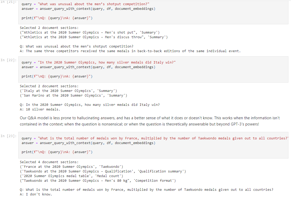
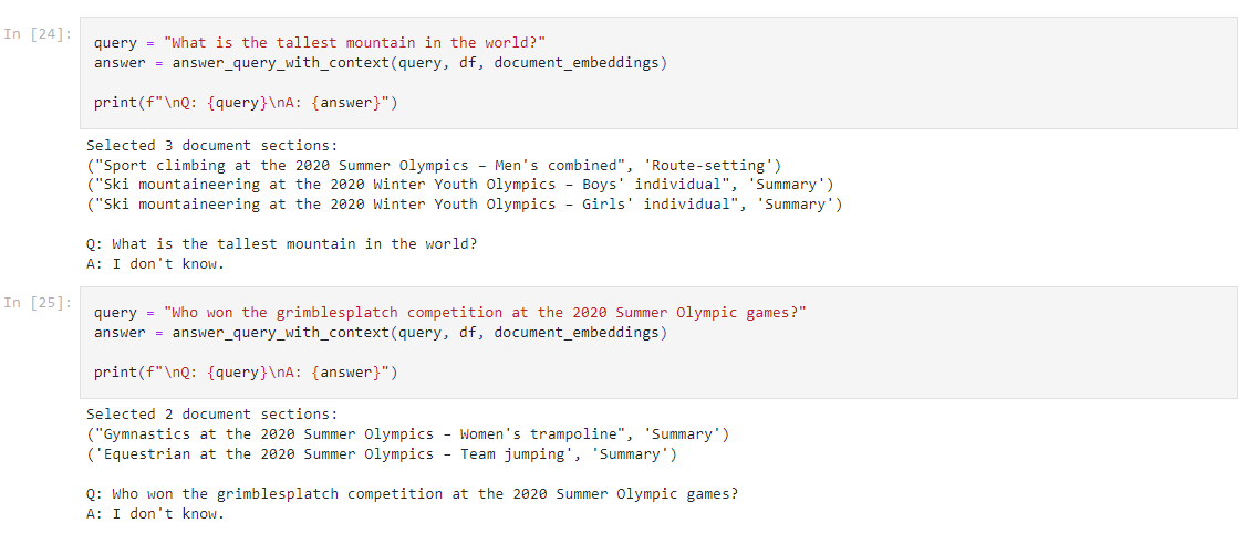
이 request 수 제한은 API 관리하는 일반적인 관행입니다. 이것을 관리하는 이유는 몇가지 있습니다.
* 첫번째로는 API 남용과 오용으로부터 시스템을 보호하는데 도움을 줍니다. 예를 들어 악의적인 의도를 가지고 API에 과부하를 일으키거나 서비스를 중단시키려는 의도로 API 요청을 다량 발생 시킬 수 있습니다. 이런 악의적인 공격으로 부터 OpenAI API 서비스를 보호하기 위해 Request 수 제한 정책이 필요합니다.
* 둘째로는 이 OpenAI API 자원을 다양한 사람이 공평하게 사용할 수 있도록 하는 목적이 있습니다. 한 개인이나 조직이 과도한 수의 요청을 하면 다른 소비자들의 API 서비스가 중단 될 수 있습니다. 단일 사용자가 만들 수 있는 요청 수를 제한 함으로서 이 API 서비스를 더 많은 사람들이 속도 저하 없이 API를 사용할 수 있는 기회를 더 보장할 수 있습니다.
* 세번째 마지막으로 이 요청량 제한은 OpenAI 가 인프라의 총 부하를 관리하는데 도움이 될 수 있습니다. API에 대한 요청이 급격하게 증가하면 서버에 부담을 주고 성능에 문제를 일으킬 수 있습니다. 이 요청량 베한을 설정함으로서 OpenAI는 모든 사용자에게 원활하고 일관된 경험을 유지하는데 도움을 줄 수 있습니다.
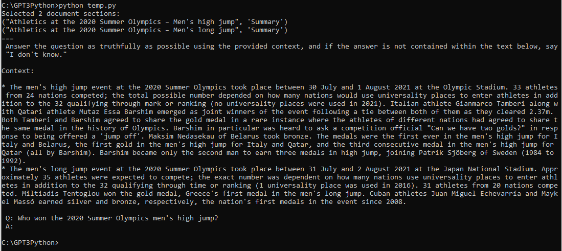
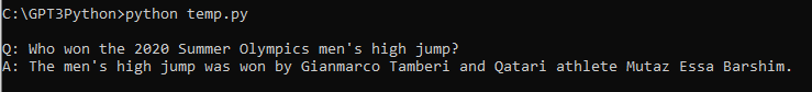
API 요청들이 너무 빨리 보내지면 아래 요청량 제한 에러가 발생합니다. OpenAI 파이썬 라이브러리를 사용한다면 그 에러 메세지는 아래와 같을 겁니다.
아래 코드는 요청량 제한을 초과하는 한 예를 보여 줍니다.
import openai  # for making OpenAI API requests

# request a bunch of completions in a loop
for _ in range(100):
    openai.Completion.create(
        model="code-cushman-001",
        prompt="def magic_function():\n\t",
        max_tokens=10,
    )
저는 굳이 이 코드는 실행해 보지 않겠습니다.
코드는 그냥 간단합니다. max_tokens를 10으로 설정한 다음에 Completion.create() api를 100번 요청하는 for 문 입니다.
How to avoid rate limit errors
Retrying with exponential backoff
이 요청량 제한 오류를 방지하는 쉬운 방법 중 하나는 random exponential backoff로 요청을 자동적으로 재 시도 하는 겁니다.
exponential backoff로 retry를 한다는 의미는 요청량 제한 에러에 도달했을 때 잠시 쉬었다가 실패한 요청을 다시 요청한다는 겁니다. 만약 그 요청이 또다시 실패 한다면 잠시 쉬는 시간이 좀 더 늘어나고 그 다음에 요청하는 과정을 반복하는 겁니다. 이 과정은 요청이 성공할 때까지 이루어지게 할 수도 있고 특정 시도 횟수를 지정해서 그 횟수 만큼만 실행하게 할 수도 있습니다.
이 접근법은 다음과 같은 이점이 있습니다.
* 자동재시도는 crash나 데이터 손실 없이 요청량 제한 에러를 극복할 수 있다는 의미입니다.
* Exponential backoff는 첫번째 시도를 빠르게 시도할 수 있음을 의미하며 처음 몇번의 재시도가 실패할 경우 점점 더 재시도까지의 쉬는 시간이 점점 더 길어진다는 겁니다. 그렇기 때문에 초기에 성공하면 좀 더 빠른 시간안에 에러를 복구 할 수 있습니다.
* Random jitter를 추가하면 동시에 모든 hitting으로부터 재시도를 하는데 도움을 줍니다.
Note. 실패한 요청은 여러분의 per-minute limit에 포함 되므로 계속 재시도를 해도 작동하지 않을 수 있습니다.
아래에 이 방법을 이용하는 몇가지 방법을 소개합니다.
Example #1: Using the Tenacity library
Tenacity 는 파이썬으로 작성된 아파치 2.0 라이센스 범용 retrying 라이브러리 입니다. 이것을 이용하면 거의 모든 상황에 재시도 동작을 추가하는 작업을 단순화 할 수 있습니다.
요청에 exponential backoff를 추가하려면 tenacity.retrydecorator를 사용하면 됩니다.
tenacity.wait_random_exponential 함수를 사용하여 random exponential backoff를 요청에 추가하는 방법을 아래 예제에서 보여 줍니다.
Note : Tenacity 라이브러리는 별도로 개발한 회사가 있고 그 회사가 배포한 라이브러리 입니다. OpenAI에서 그 안정성이나 보안을 보장하지는 않습니다.
import openai  # for OpenAI API calls
from tenacity import (
    retry,
    stop_after_attempt,
    wait_random_exponential,
)  # for exponential backoff


@retry(wait=wait_random_exponential(min=1, max=60), stop=stop_after_attempt(6))
def completion_with_backoff(**kwargs):
    return openai.Completion.create(**kwargs)


completion_with_backoff(model="text-davinci-002", prompt="Once upon a time,")
@retry() 를 사용하며 wait과 stop을 지정합니다.
재시도 사이 대기시간이 1초에서 60초 사이가 되고 재시도는 6번 시도하라는 겁니다.
이것은 그 아래 함수인 Completion_with_backoff() 함수에 적용 됩니다.
Tenacity와 마찬가지로 Backoff 라이브러리는 third-party tool 입니다. OpenAI에서 그 안정성이나 보안성을 보장하지는 않습니다.
import backoff  # for exponential backoff
import openai  # for OpenAI API calls


@backoff.on_exception(backoff.expo, openai.error.RateLimitError)
def completions_with_backoff(**kwargs):
    return openai.Completion.create(**kwargs)


completions_with_backoff(model="text-davinci-002", prompt="Once upon a time,")
이런 3rd-party 툴을 사용하지 않고 직접 backoff 로직을 구현할 수도 있습니다.
# imports
import random
import time

import openai

# define a retry decorator
def retry_with_exponential_backoff(
    func,
    initial_delay: float = 1,
    exponential_base: float = 2,
    jitter: bool = True,
    max_retries: int = 10,
    errors: tuple = (openai.error.RateLimitError,),
):
    """Retry a function with exponential backoff."""

    def wrapper(*args, **kwargs):
        # Initialize variables
        num_retries = 0
        delay = initial_delay

        # Loop until a successful response or max_retries is hit or an exception is raised
        while True:
            try:
                return func(*args, **kwargs)

            # Retry on specified errors
            except errors as e:
                # Increment retries
                num_retries += 1

                # Check if max retries has been reached
                if num_retries > max_retries:
                    raise Exception(
                        f"Maximum number of retries ({max_retries}) exceeded."
                    )

                # Increment the delay
                delay *= exponential_base * (1 + jitter * random.random())

                # Sleep for the delay
                time.sleep(delay)

            # Raise exceptions for any errors not specified
            except Exception as e:
                raise e

    return wrapper


@retry_with_exponential_backoff
def completions_with_backoff(**kwargs):
    return openai.Completion.create(**kwargs)


completions_with_backoff(model="text-davinci-002", prompt="Once upon a time,")
이 에제를 보면 위에서 설명했던 동작인 요청하고 error가 발생하면 재시도를 정해진 횟수만큼 하고 그 재시도 사이의 지연 시간은 점차 증가해 나가는 동작을 하도록 직접 wrapper() 함수 안에 구현을 해 놨습니다.
그리고 최대 재시도 횟수와 지연시간 관련 값들은 retry_with_exponential_backoff() 함수에서 세팅을 했습니다.
그리고 위에 설명한 wrapper() 함수는 이 retry_with_exponential_backoff() 함수에 속해 있습니다.
How to maximize throughput of batch processing given rate limits
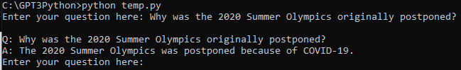
만약 여러분의 애플리케이션이 고객의 실시간 요청을 처리하는 서비스를 제공한다면 backoff and retry는 요청량 제한 에러를 피하면서 latency를 minimize할 수 있는 아주 좋은 전략입니다.
그런데 이렇게 서비스 제공 시간이 중요한게 아니라 얼마나 많은 양을 처리하느냐가 더 중요한 애플리케이션이 있을 수 있습니다. 대량의 batch data를 처리하는 것이 더 중요한 경우이죠. 이런 경우 backoff and retry 말고 여러분이 사용할 수 있는 몇가지 다른 방법이 있습니다.
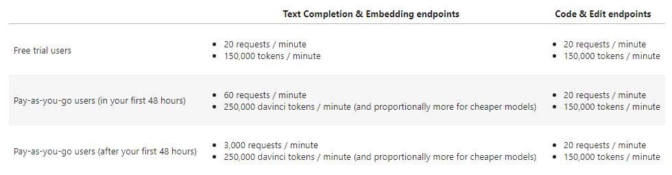
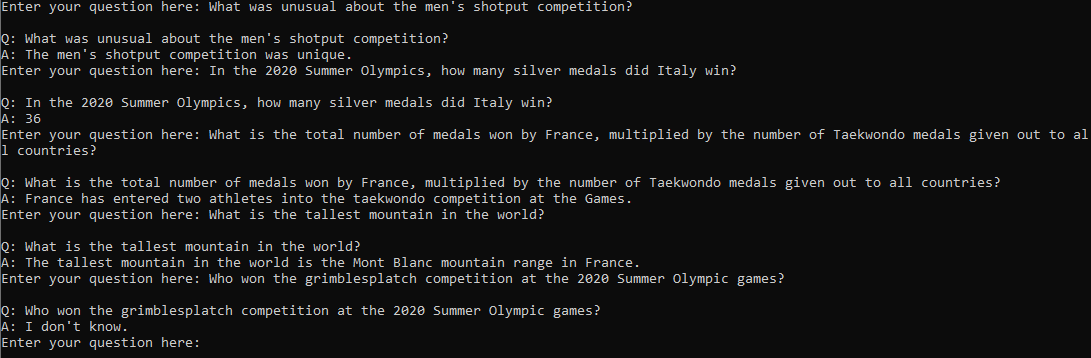
Proactively adding delay between requests
만약 여러분의 앱이 요청량 제한에 걸리고 back off 하고 재시도하고 하는 상황이 계속 반복 되면서 금방 요청량 제한에 걸린다면 남아 있는 시간은 제한량 초과 메세지만 받으면서 요청을 계속 할 수 있습니다. (예를 들어 1분에 20회가 제한량인데 이 20회가 10초만에 도달하면 나머지 50초는 제한량 초과 메세지만 받게 될 것입니다.) 그러면 이 50초 동안의 요청은 낭비 되는 것이죠. 그것을 하기 위해 사용한 내 시스템의 리소스가 낭비 되는 것입니다.
이 경우 잠재적 해결책이 될 수 있는 것은 여러분의 요청량 제한을 계산하고 그 reciprocal에 맞게 지연 시간을 만드는 것입니다.
reciprocal(예: 만약 여러분의 요청량 제한이 분당 20이라면 각 request마다 지연시간을 3~6초씩 추가 해 주는 것)
이렇게 하면 요청량 제한의 상한선에 도달하지 않고 낭비되는 요청도 발생 시키지 않는 상황에 가깝게 만들 수 있습니다.
Example of adding delay to a request
# imports
import time
import openai

# Define a function that adds a delay to a Completion API call
def delayed_completion(delay_in_seconds: float = 1, **kwargs):
    """Delay a completion by a specified amount of time."""

    # Sleep for the delay
    time.sleep(delay_in_seconds)

    # Call the Completion API and return the result
    return openai.Completion.create(**kwargs)


# Calculate the delay based on your rate limit
rate_limit_per_minute = 20
delay = 60.0 / rate_limit_per_minute

delayed_completion(
    delay_in_seconds=delay,
    model="text-davinci-002",
    prompt="Once upon a time,"
)
이 소스 코드는 위에 예시로 들었던 상황에 맞게 만든 겁니다.
요청량 제한이 분당 20이라면 delay는 60/20 즉 3초가 됩니다.
delay_completion() 함수 안데 time.sleep() 을 이 3초로 했기 때문에 이 함수를 호출할 때 마다 3초씩 기다렸다가 openai.Completion.create() api 를 사용하게 되는 겁니다.
그러면 이 1분이라는 시간에 할 수 있는 요청량을 최대한으로 사용할 수 있게 됩니다.
단 10초만에 요청량 제한에 걸려서 나머지 50초는 그냥 손 놓고 있는 상황을 피할 수 있게 되는 거죠.
Batching requests
OpenAI api에는 분당 요청량 제한 이외에 분당 요청 토큰에 대한 별도의 제한이 있습니다.
만약 여러분이 분당 요청량 제한에 도달했지만 분당 토큰에 여유가 있는 경우 각 요청에 여러 작업을 batch 함으로서 throughput(처리량)을 증가시킬 수 있습니다.
프롬프트들의 batch를 보내는 방법은 일반적인 API 콜과 동일하게 작동합니다.
단지 프롬프트 파라미터가 Single string이 아니라 String 의 List라는 것만 다릅니다.
Warning: Response 는 그 prompt 의 순서대로 반환을 하지 않을 수 있습니다. 그렇기 때문에 index 필드를 사용하여 그 response를 prompt 의 파라미터 순서와 맞게 일치시키는 작업을 반드시 해야 합니다.
Example without batching
import openai  # for making OpenAI API requests


num_stories = 10
prompt = "Once upon a time,"

# serial example, with one story completion per request
for _ in range(num_stories):
    response = openai.Completion.create(
        model="curie",
        prompt=prompt,
        max_tokens=20,
    )

    # print story
    print(prompt + response.choices[0].text)
Example with batching
import openai  # for making OpenAI API requests


num_stories = 10
prompts = ["Once upon a time,"] * num_stories

# batched example, with 10 stories completions per request
response = openai.Completion.create(
    model="curie",
    prompt=prompts,
    max_tokens=20,
)

# match completions to prompts by index
stories = [""] * len(prompts)
for choice in response.choices:
    stories[choice.index] = prompts[choice.index] + choice.text

# print stories
for story in stories:
    print(story)
위의 예제는 prompt 'once upon a time' 단일 파라미터로 하는 openai.Completion.create() 호출을 for 문을 통해서 10번 일으켰습니다.
즉 10번 요청을 한 것입니다.
그런데 두번째 예제는 prompt 자체를 Once upon a time이 10번 들어가 있는 리스트로 만든 다음 이 리스트를 파라미터로 전달해서 openai.Completion.create() api를 호출 했습니다.
즉 1번 요청한 것입니다.
이렇게 함으로서 요청량을 줄일 수 있게 되는 것입니다.
두번째 예제의 첫번째 for 문에서는 response를 request의 index 와 맞게 매치 시키는 작업을 하고 있습니다.
그래서 질문 + 응답 이런 식으로 stories[] 에 저장되게 했습니다.
이제 이 stories[]를 두번째 for 문처럼 print 하기만 하면 해당 질문과 그에 대한 답변 식으로 출력이 됩니다.
Example parallel processing script
대량의 API 요청을 parallel (병렬) 처리하기 위한 예제 스크립트는 아래에 있습니다.
오늘 예제는 이 모델의 최대 context 길이보다 더 긴 텍스트는 어떻게 처리를 해야 하는지를 보여 줍니다.
1. Model context length
import openai
from tenacity import retry, wait_random_exponential, stop_after_attempt, retry_if_not_exception_type
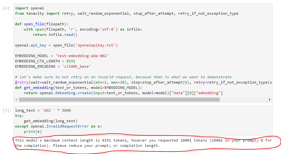
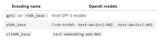
EMBEDDING_MODEL = 'text-embedding-ada-002'
EMBEDDING_CTX_LENGTH = 8191
EMBEDDING_ENCODING = 'cl100k_base'
# let's make sure to not retry on an invalid request, because that is what we want to demonstrate
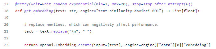
@retry(wait=wait_random_exponential(min=1, max=20), stop=stop_after_attempt(6), retry=retry_if_not_exception_type(openai.InvalidRequestError))
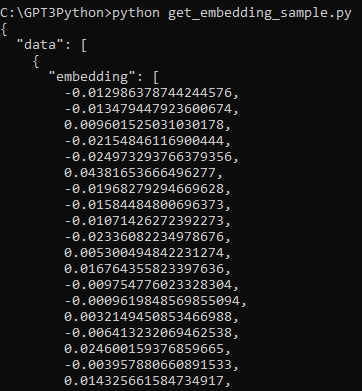
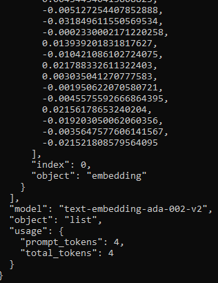
def get_embedding(text_or_tokens, model=EMBEDDING_MODEL):
return openai.Embedding.create(input=text_or_tokens, model=model)["data"][0]["embedding"]
가장 먼저 openai를 import 하고 그 다음에 tenacity 모듈을 import 합니다.
tenacity는 런타임 중 오류가 발생해서 종료가 될 때 이 종료하는 것을 막고 다시 retry 하고자 할 때 사용하는 파이썬 모듈입니다.
이 모듈 중에서 retry, wait_random_exponential, Stop_after_attempt, retry_if_not_exception_type 만 import 합니다.
(이렇게 하면 @tenacity.retry 라고 하지 않고 간단하게 @retry 형식으로 사용할 수 있습니다.)
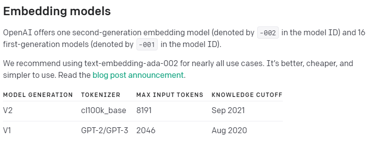
그 다음은 openai 모델을 설정하고 context length 를 8191 로 지정하고 encoding은 cl100k_base 로 합니다.
cl100k_base 는 tokenizer로 Max Input Token은 8191 로 정해져 있습니다. 2021년 9월에 발표 됐습니다.
자세한 내용은 OpenAI Guide의 Embeddings Overview 페이지를 참조하세요.
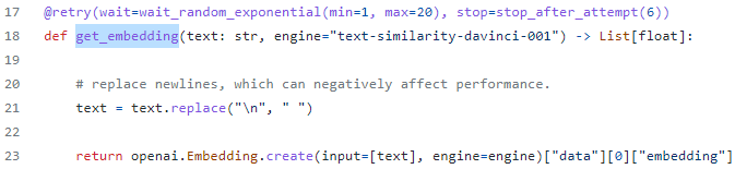
그 다음 은 @retry 구문이 나옵니다. retry 사이에 기다리는 시간은 1~20초이고 6번 까지 시도하고 exception type이 InvalidRequestError 가 아닌 경우만 retry를 시도합니다. InvalidRequest인 경우는 Retry를 해도 아무 소용 없으니까요.
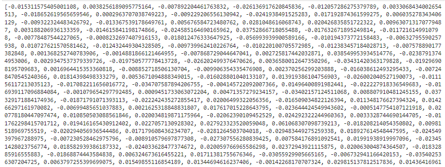
그 다음은 get_embedding() 함수를 만들었습니다.
입력 파라미터로는 text_or_tokens와 모델 이름을 받습니다.
그리고 이 입력값에 대한 embedding 값을 전달받은 모델을 사용해서 openai.Embedding.create() api로 부터 받고 그 값을 return 합니다.
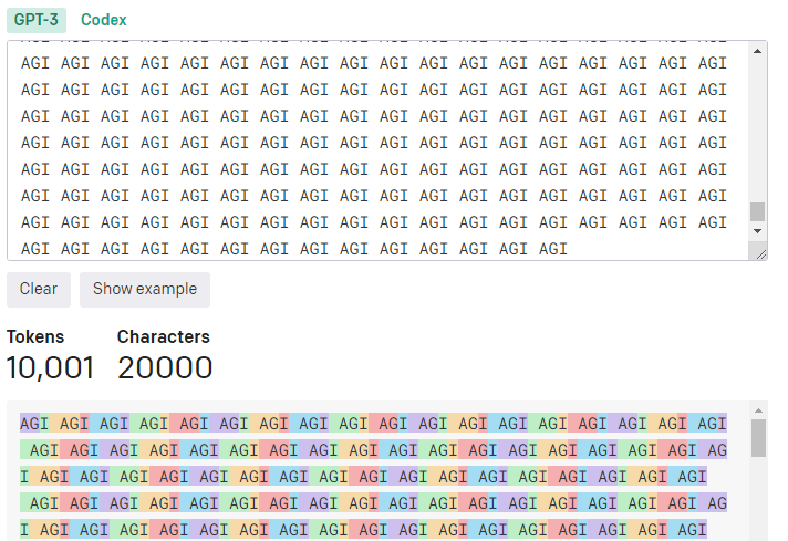
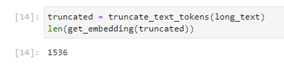
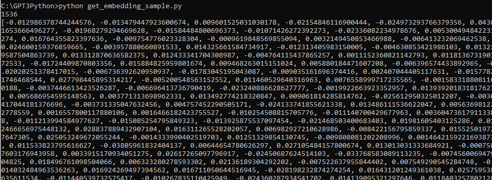
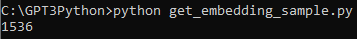
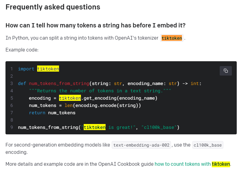
여기서 크기는 토큰으로 정해지기 때문에 먼저 입력값이 몇개의 토큰으로 이루어져 있는지 알아봐야 합니다.
위 Tokenizer 페이지에서 그 작업을 했었죠. 10001 이었습니다. 그리고 위에서 사용한 모델은 8191 개의 토큰이 입력 허용 최대값이구요.
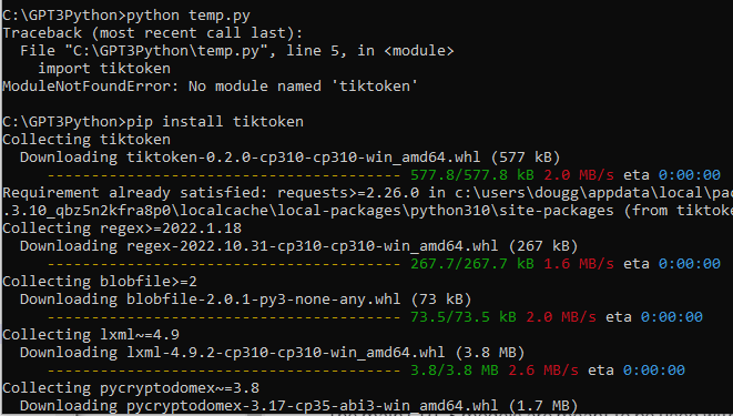
아래 방법이 이렇게 입력값을 토큰화 해서 자르는 부분입니다.
import tiktoken

def truncate_text_tokens(text, encoding_name=EMBEDDING_ENCODING, max_tokens=EMBEDDING_CTX_LENGTH):
    """Truncate a string to have `max_tokens` according to the given encoding."""
    encoding = tiktoken.get_encoding(encoding_name)
    return encoding.encode(text)[:max_tokens]
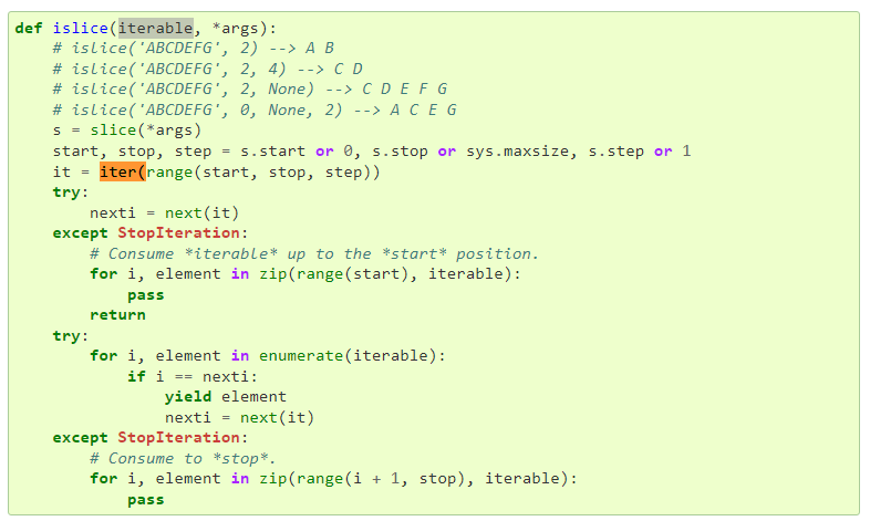
from itertools import islice

def batched(iterable, n):
    """Batch data into tuples of length n. The last batch may be shorter."""
    # batched('ABCDEFG', 3) --> ABC DEF G
    if n < 1:
        raise ValueError('n must be at least one')
    it = iter(iterable)
    while (batch := tuple(islice(it, n))):
        yield batch
우선 itertools 의 islice 함수를 import 합니다.
그리고 batched() 함수를 만들고 입력값으로는 iterable과 n을 받습니다.
그 다음 입력 받은 데이터를 길이가 n인 tuple로 batch 처리 합니다. 마지막 batch는 길이가 n 보다 작을 수 있습니다.
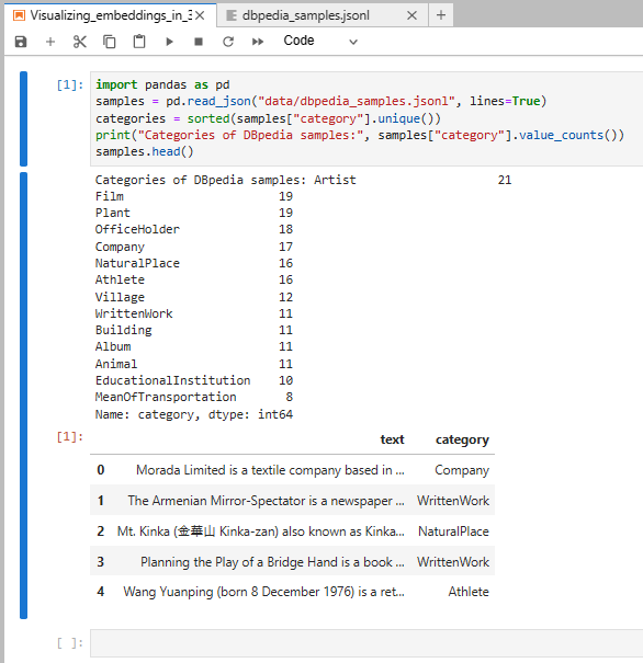
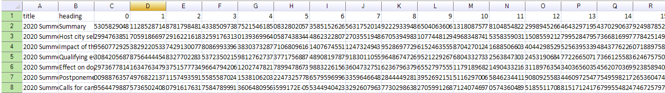
{"text": " Morada Limited is a textile company based in Altham Lancashire. Morada specializes in curtains.", "category": "Company"} {"text": " The Armenian Mirror-Spectator is a newspaper published by the Baikar Association in Watertown Massachusetts.", "category": "WrittenWork"}
text 와 category 두 항목이 있습니다.
text는 한 문장이 있고 category에는 말 그대로 카테고리들이 있습니다.
어떤 카테고리들이 있고 각 카테고리는 몇개씩 있는지 알아 보겠습니다.
여기서는 pandas 모듈을 사용합니다.
read_json()을 사용해서 데이터세트를 읽어 옵니다. (samples)
그리고 이 데이터세트의 category를 수집해서 unique 한 리스트를 만든 후 정렬을 합니다. (categories)
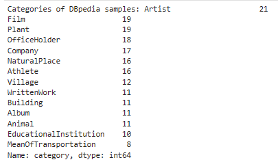
print("Categories of DBpedia samples:", samples["category"].value_counts())
이것을 위 방식으로 프린트를 하면 이런 결과를 얻습니다.
카테고리는 총 14개가 있고 그 중에 가장 많이 있는 카테고리는 Artist 로 21번 나옵니다.
그 외에 다른 카테고리들과 각 카테고리별 갯수를 표시합니다.
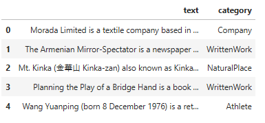
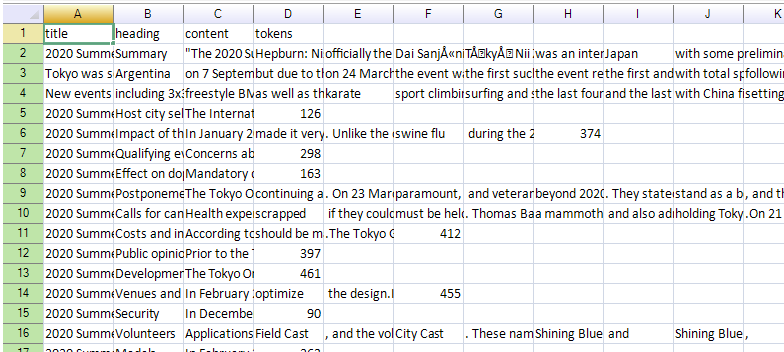
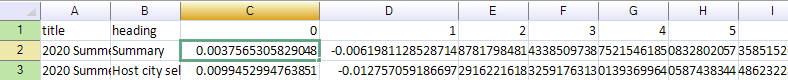
그리고 samples.head() 를 하면 아래 결과를 얻습니다.
text와 category를 표 형식으로 보여 줍니다. head()를 사용하면 디폴트로 상위 5줄을 print 합니다.
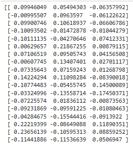
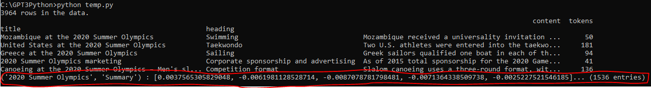
그 다음은 openai api를 이용해서 각 text별로 임베딩 값을 받아 옵니다.
import openai
from openai.embeddings_utils import get_embeddings
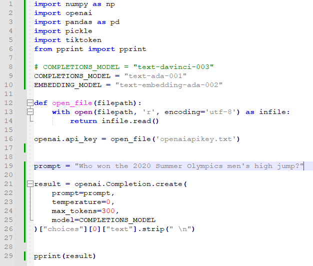
def open_file(filepath):
with open(filepath, 'r', encoding='utf-8') as infile:
return infile.read()
openai.api_key = open_file('openaiapikey.txt')
# NOTE: The following code will send a query of batch size 200 to /embeddings
matrix = get_embeddings(samples["text"].to_list(), engine="text-embedding-ada-002")
embeddings_utils 의 get_embeddings를 사용해서 각 text 별로 openai로 부터 임베딩 값을 받아 옵니다.
Note : openai api는 유료입니다. 200개의 데이터에 대한 임베딩값을 받아오는데 대한 과금이 붙습니다.
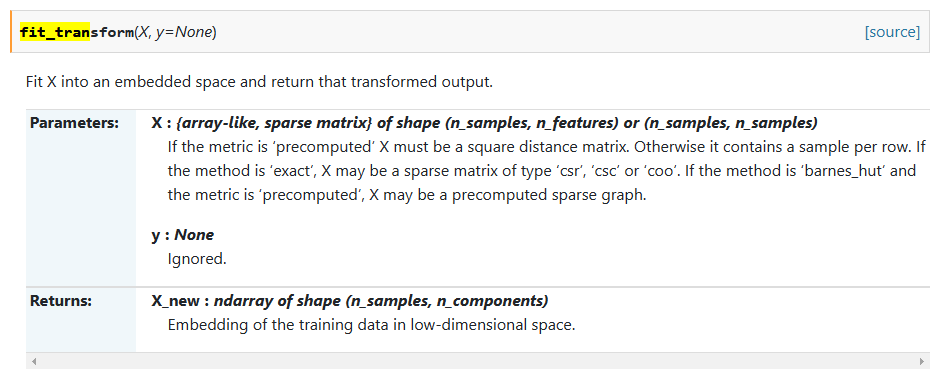
t-SNE decomposition (분해)를 사용해서 dimensionality를 2차원으로 줄입니다.
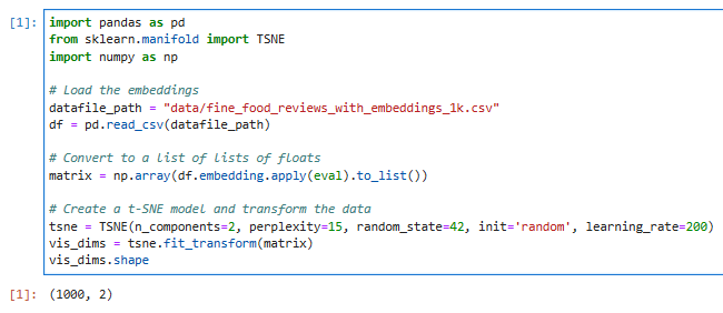
import pandas as pd
from sklearn.manifold import TSNE
import numpy as np
# Load the embeddings
datafile_path = "data/fine_food_reviews_with_embeddings_1k.csv"
df = pd.read_csv(datafile_path)
# Convert to a list of lists of floats
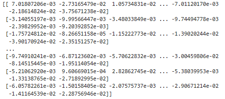
matrix = np.array(df.embedding.apply(eval).to_list())
# Create a t-SNE model and transform the data
tsne = TSNE(n_components=2, perplexity=15, random_state=42, init='random', learning_rate=200)
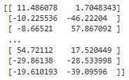
vis_dims = tsne.fit_transform(matrix)
vis_dims.shape
모듈은 pandas, numpy 그리고 sklearn.manifold의 TSNE를 사용합니다.
모두 이전 글에서 배운 모듈들 입니다.
판다스의 read_csv() 함수를 사용해서 csv 데이터 파일을 읽습니다.
그 다음 numpy 의 array()를 사용해서 csv 파일의 embedding 컬럼에 있는 값들을 리스트 형식으로 변환합니다.
이 값을 shape을 이용해서 리스트의 크기와 차원을 표시하면 위에 처럼 1000,2 라고 나옵니다.
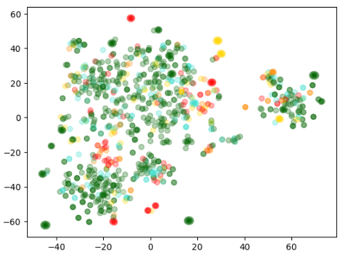
2. Plotting the embeddings
위에서 처럼 2차원으로 데이터를 정리하면 2D 산점도 분포도를 그릴 수 있다고 했습니다.
아래에서는 그것을 그리기 전에 알아보기 쉽도록 각 review에 대한 색을 지정해서 알아보기 쉽도록 합니다.
이 색은 별점 점수와 ranging 데이터를 기반으로 빨간색에서 녹색에 걸쳐 표현됩니다.
import matplotlib.pyplot as plt
import matplotlib
import numpy as np
colors = ["red", "darkorange", "gold", "turquoise", "darkgreen"]
x = [x for x,y in vis_dims]
y = [y for x,y in vis_dims]
color_indices = df.Score.values - 1
colormap = matplotlib.colors.ListedColormap(colors)
plt.scatter(x, y, c=color_indices, cmap=colormap, alpha=0.3)
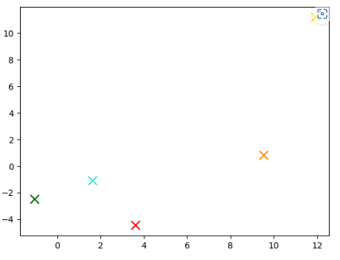
for score in [0,1,2,3,4]:
avg_x = np.array(x)[df.Score-1==score].mean()
avg_y = np.array(y)[df.Score-1==score].mean()
color = colors[score]
plt.scatter(avg_x, avg_y, marker='x', color=color, s=100)
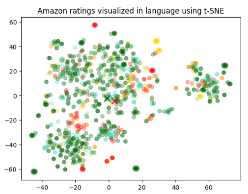
plt.title("Amazon ratings visualized in language using t-SNE")
그리고 plt.title()에서 이 표의 제목을 정해주면 결과와 같은 그림을 얻을 수 있습니다.
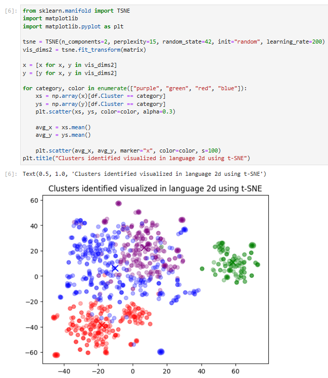
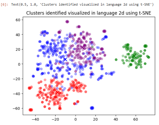
4개의 그룹중에 녹색 그룹은 다른 그룹들과 좀 동떨어져 있는 것을 보실 수 있습니다.
2. Text samples in the clusters & naming the clusters
지금까지는 raw data를 clustering 하는 법과 이 clustering 한 데이터를 시각화 해서 보여주는 방법을 보았습니다.
이제 openai의 api를 이용해서 각 클러스터의 랜덤 샘플들을 보여 주는 코드입니다.
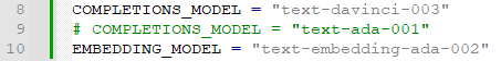
openai.Completion.create() api를 사용할 것이고 모델 (engine)은 text-ada-001을 사용합니다.
prompt는 아래 질문 입니다.
What do the following customer reviews have in common?
그러면 각 클러스터 별로 review 를 분석한 값들이 response 됩니다.
우선 아래 코드를 실행 해 보겠습니다.
import openai

def open_file(filepath):
    with open(filepath, 'r', encoding='utf-8') as infile:
        return infile.read()

openai.api_key = open_file('openaiapikey.txt')

# Reading a review which belong to each group.
rev_per_cluster = 5

for i in range(n_clusters):
    print(f"Cluster {i} Theme:", end=" ")

    reviews = "\n".join(
        df[df.Cluster == i]
        .combined.str.replace("Title: ", "")
        .str.replace("\n\nContent: ", ":  ")
        .sample(rev_per_cluster, random_state=42)
        .values
    )
    response = openai.Completion.create(
        engine="text-ada-001",  #"text-davinci-003",
        prompt=f'What do the following customer reviews have in common?\n\nCustomer reviews:\n"""\n{reviews}\n"""\n\nTheme:',
        temperature=0,
        max_tokens=64,
        top_p=1,
        frequency_penalty=0,
        presence_penalty=0,
    )
    print(response)
openai를 import 하고 openai api key를 제공하는 부분으로 시작합니다.
그리고 rev_per_cluster는 5로 합니다.
그 다음 for 문에서 n_clusters만큼 루프를 도는데 위에서 n_clusters는 4로 설정돼 있었습니다.
reviews에는 Title과 Content 내용을 넣는데 샘플로 5가지를 무작위로 뽑아서 넣습니다.
그리고 이 reviews 값을 prompt에 삽입해서 openai.Completion.create() api로 request 합니다.
그러면 이 prompt에 대한 response 가 response 변수에 담깁니다.
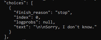
이 response 만 우선 출력해 보겠습니다.
Cluster 0 Theme: {
"choices": [
{
"finish_reason": "stop",
"index": 0,
"logprobs": null,
"text": " Customer reviews:gluten free, healthy bars, content:\n\nThe customer reviews have in common that they save money on Amazon by ordering by themselves by looking for gluten free healthy bars. The bars are also delicious."
}
],
"created": 1677191195,
"id": "cmpl-6nEKppB6SqCz07LYTcaktEAgq06hm",
"model": "text-ada-001",
"object": "text_completion",
"usage": {
"completion_tokens": 44,
"prompt_tokens": 415,
"total_tokens": 459
}
}
Cluster 1 Theme: {
"choices": [
{
"finish_reason": "stop",
"index": 0,
"logprobs": null,
"text": " Cat food\n\nMessy, undelicious, and possibly unhealthy."
}
],
"created": 1677191195,
"id": "cmpl-6nEKpGffRc2jyJB4gNtuCa09dG2GT",
"model": "text-ada-001",
"object": "text_completion",
"usage": {
"completion_tokens": 15,
"prompt_tokens": 529,
"total_tokens": 544
}
}
Cluster 2 Theme: {
"choices": [
{
"finish_reason": "stop",
"index": 0,
"logprobs": null,
"text": " Coffee\n\nThe customer's reviews have in common that they are among the best in the market, Rodeo Drive, and that the customer is able to enjoy their coffee half and half because they have an Amazon account."
}
],
"created": 1677191196,
"id": "cmpl-6nEKqxza0t8vGRAiK9K5RtCy3Gwbl",
"model": "text-ada-001",
"object": "text_completion",
"usage": {
"completion_tokens": 45,
"prompt_tokens": 443,
"total_tokens": 488
}
}
Cluster 3 Theme: {
"choices": [
{
"finish_reason": "stop",
"index": 0,
"logprobs": null,
"text": " Customer reviews of different brands of soda."
}
],
"created": 1677191196,
"id": "cmpl-6nEKqKuxe4CVJTV4GlIZ7vxe6F85o",
"model": "text-ada-001",
"object": "text_completion",
"usage": {
"completion_tokens": 8,
"prompt_tokens": 616,
"total_tokens": 624
}
}
이 respons를 보시면 각 Cluster 별로 응답을 받았습니다.
위에 for 문에서 각 클러스터별로 request를 했기 때문입니다.
이제 이 중에서 실제 질문에 대한 답변인 choices - text 부분만 뽑아 보겠습니다.
import openai
def open_file(filepath):
with open(filepath, 'r', encoding='utf-8') as infile:
return infile.read()
openai.api_key = open_file('openaiapikey.txt')
# Reading a review which belong to each group.
rev_per_cluster = 5
for i in range(n_clusters):
print(f"Cluster {i} Theme:", end=" ")
reviews = "\n".join(
df[df.Cluster == i]
.combined.str.replace("Title: ", "")
.str.replace("\n\nContent: ", ": ")
.sample(rev_per_cluster, random_state=42)
.values
)
response = openai.Completion.create(
engine="text-ada-001", #"text-davinci-003",
prompt=f'What do the following customer reviews have in common?\n\nCustomer reviews:\n"""\n{reviews}\n"""\n\nTheme:',
temperature=0,
max_tokens=64,
top_p=1,
frequency_penalty=0,
presence_penalty=0,
)
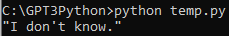
print(response["choices"][0]["text"].replace("\n", ""))
답변은 아래와 같습니다.
Cluster 0 Theme:  Customer reviews:gluten free, healthy bars, content:The customer reviews have in common that they save money on Amazon by ordering by themselves by looking for gluten free healthy bars. The bars are also delicious.
Cluster 1 Theme:  Cat foodMessy, undelicious, and possibly unhealthy.
Cluster 2 Theme:  CoffeeThe customer's reviews have in common that they are among the best in the market, Rodeo Drive, and that the customer is able to enjoy their coffee half and half because they have an Amazon account.
Cluster 3 Theme:  Customer reviews of different brands of soda.
Cluster 0 Theme:      Unnamed: 0   ProductId          UserId  Score  \
117         400  B008JKU2CO  A1XV4W7JWX341C      5
25          274  B008JKTH2A  A34XBAIFT02B60      1
722         534  B0064KO16O  A1K2SU61D7G41X      5
289           7  B001KP6B98   ABWCUS3HBDZRS      5
590         948  B008GG2N2S  A1CLUIIJL6EHLU      5

                                               Summary  \
117  Loved these gluten free healthy bars, saved $$...
25   Should advertise coconut as an ingredient more...
722                                        very good!!
289                                  Excellent product
590                                          delicious

                                                  Text  \
117  These Kind Bars are so good and healthy & glut...
25   First, these should be called Mac - Coconut ba...
722  just like the runts<br />great flavor, def wor...
289  After scouring every store in town for orange ...
590  Gummi Frogs have been my favourite candy that ...

                                              combined  n_tokens  \
117  Title: Loved these gluten free healthy bars, s...        96
25   Title: Should advertise coconut as an ingredie...        78
722  Title: very good!!; Content: just like the run...        43
289  Title: Excellent product; Content: After scour...       100
590  Title: delicious; Content: Gummi Frogs have be...        75

                                             embedding  Cluster
117  [-0.002289338270202279, -0.01313735730946064, ...        0
25   [-0.01757248118519783, -8.266511576948687e-05,...        0
722  [-0.011768403463065624, -0.025617636740207672,...        0
289  [0.0007493243319913745, -0.017031244933605194,...        0
590  [-0.005802689120173454, 0.0007485789828933775,...        0
Cluster 1 Theme:      Unnamed: 0   ProductId          UserId  Score  \
536         731  B0029NIBE8  A3RKYD8IUC5S0N      2
332         184  B000WFRUOC   A22RVTZEIVHZA      4
424         153  B0007A0AQW  A15X1BO4CLBN3C      5
298          24  B003R0LKRW  A1OQSU5KYXEEAE      1
960         589  B003194PBC  A2FSDQY5AI6TNX      5

                              Summary  \
536  Messy and apparently undelicious
332                  The cats like it
424          cant get enough of it!!!
298               Food Caused Illness
960          My furbabies LOVE these!

                                                  Text  \
536  My cat is not a huge fan. Sure, she'll lap up ...
332  My 7 cats like this food but it is a little yu...
424  Our lil shih tzu puppy cannot get enough of it...
298  I switched my cats over from the Blue Buffalo ...
960  Shake the container and they come running. Eve...

                                              combined  n_tokens  \
536  Title: Messy and apparently undelicious; Conte...       181
332  Title: The cats like it; Content: My 7 cats li...        87
424  Title: cant get enough of it!!!; Content: Our ...        59
298  Title: Food Caused Illness; Content: I switche...       131
960  Title: My furbabies LOVE these!; Content: Shak...        47

                                             embedding  Cluster
536  [-0.002376032527536154, -0.0027701142244040966...        1
332  [0.02162935584783554, -0.011174295097589493, -...        1
424  [-0.007517425809055567, 0.0037251529283821583,...        1
298  [-0.0011128562036901712, -0.01970377005636692,...        1
960  [-0.009749102406203747, -0.0068712360225617886...        1
Cluster 2 Theme:      Unnamed: 0   ProductId          UserId  Score  \
135         410  B007Y59HVM  A2ERWXZEUD6APD      5
439         812  B0001UK0CM  A2V8WXAFG1TEOC      5
326         107  B003VXFK44  A21VWSCGW7UUAR      4
475         852  B000I6MCSY   AO34Q3JGZU0JQ      5
692         922  B003TC7WN4  A3GFZIL1E0Z5V8      5

                               Summary  \
135                  Fog Chaser Coffee
439                    Excellent taste
326   Good, but not Wolfgang Puck good
475             Just My Kind of Coffee
692  Rodeo Drive is Crazy Good Coffee!

                                                  Text  \
135  This coffee has a full body and a rich taste. ...
439  This is to me a great coffee, once you try it ...
326  Honestly, I have to admit that I expected a li...
475  Coffee Masters Hazelnut coffee used to be carr...
692  Rodeo Drive is my absolute favorite and I'm re...

                                              combined  n_tokens  \
135  Title: Fog Chaser Coffee; Content: This coffee...        42
439  Title: Excellent taste; Content: This is to me...        31
326  Title: Good, but not Wolfgang Puck good; Conte...       178
475  Title: Just My Kind of Coffee; Content: Coffee...       118
692  Title: Rodeo Drive is Crazy Good Coffee!; Cont...        59

                                             embedding  Cluster
135  [0.006498195696622133, 0.006776264403015375, 0...        2
439  [0.0039436533115804195, -0.005451332312077284,...        2
326  [-0.003140551969408989, -0.009995664469897747,...        2
475  [0.010913548991084099, -0.014923149719834328, ...        2
692  [-0.029914353042840958, -0.007755572907626629,...        2
Cluster 3 Theme:      Unnamed: 0   ProductId          UserId  Score  \
495         831  B0014X5O1C   AHYRTWABDAG1H      5
978         642  B00264S63G  A36AUU1UNRS48G      5
916         686  B008PYVINQ  A1DRWYIO7JN1MD      2
696         926  B0062P9XPU  A33KQALCZGXG8C      5
491         828  B000EIE20M  A39QHSDUBR8L0T      3

                               Summary  \
495  Wonderful alternative to soda pop
978      So convenient, for so little!
916                    bot very cheesy
696                         Delicious!
491                            Just ok

                                                  Text  \
495  This is a wonderful alternative to soda pop.  ...
978  I needed two vanilla beans for the Love Goddes...
916  Got this about a month ago.first of all it sme...
696  I am not a huge beer lover.  I do enjoy an occ...
491  I bought this brand because it was all they ha...

                                              combined  n_tokens  \
495  Title: Wonderful alternative to soda pop; Cont...       273
978  Title: So convenient, for so little!; Content:...       121
916  Title: bot very cheesy; Content: Got this abou...        46
696  Title: Delicious!; Content: I am not a huge be...        97
491  Title: Just ok; Content: I bought this brand b...        58

                                             embedding  Cluster
495  [0.022326279431581497, -0.018449820578098297, ...        3
978  [-0.004598899278789759, -0.01737511157989502, ...        3
916  [-0.010750919580459595, -0.0193503275513649, -...        3
696  [0.009483409114181995, -0.017691848799586296, ...        3
491  [-0.0023960231337696314, -0.006881058216094971...        3
여기서 데이터를 아래와 같이 가공을 합니다.
    for j in range(rev_per_cluster):
        print(sample_cluster_rows.Score.values[j], end=", ")
        print(sample_cluster_rows.Summary.values[j], end=":   ")
        print(sample_cluster_rows.Text.str[:70].values[j])
Score의 값들을 가지고 오고 끝에는 쉼표 , 를 붙입니다.
그리고 Summary의 값을 가지고 오고 끝에는 : 를 붙입니다.
그리고 Text컬럼의 string을 가지고 오는데 70자 까지만 가지고 옵니다.
전체 결과를 보겠습니다.
Cluster 0 Theme:  Customer reviews:gluten free, healthy bars, content:The customer reviews have in common that they save money on Amazon by ordering by themselves by looking for gluten free healthy bars. The bars are also delicious.
5, Loved these gluten free healthy bars, saved $$ ordering on Amazon:   These Kind Bars are so good and healthy & gluten free.  My daughter ca
1, Should advertise coconut as an ingredient more prominently:   First, these should be called Mac - Coconut bars, as Coconut is the #2
5, very good!!:   just like the runts<br />great flavor, def worth getting<br />I even o
5, Excellent product:   After scouring every store in town for orange peels and not finding an
5, delicious:   Gummi Frogs have been my favourite candy that I have ever tried. of co
Cluster 1 Theme:  Cat foodMessy, undelicious, and possibly unhealthy.
2, Messy and apparently undelicious:   My cat is not a huge fan. Sure, she'll lap up the gravy, but leaves th
4, The cats like it:   My 7 cats like this food but it is a little yucky for the human. Piece
5, cant get enough of it!!!:   Our lil shih tzu puppy cannot get enough of it. Everytime she sees the
1, Food Caused Illness:   I switched my cats over from the Blue Buffalo Wildnerness Food to this
5, My furbabies LOVE these!:   Shake the container and they come running. Even my boy cat, who isn't
Cluster 2 Theme:  CoffeeThe customer's reviews have in common that they are among the best in the market, Rodeo Drive, and that the customer is able to enjoy their coffee half and half because they have an Amazon account.
5, Fog Chaser Coffee:   This coffee has a full body and a rich taste. The price is far below t
5, Excellent taste:   This is to me a great coffee, once you try it you will enjoy it, this
4, Good, but not Wolfgang Puck good:   Honestly, I have to admit that I expected a little better. That's not
5, Just My Kind of Coffee:   Coffee Masters Hazelnut coffee used to be carried in a local coffee/pa
5, Rodeo Drive is Crazy Good Coffee!:   Rodeo Drive is my absolute favorite and I'm ready to order more!  That
Cluster 3 Theme:  Customer reviews of different brands of soda.
5, Wonderful alternative to soda pop:   This is a wonderful alternative to soda pop.  It's carbonated for thos
5, So convenient, for so little!:   I needed two vanilla beans for the Love Goddess cake that my husbands
2, bot very cheesy:   Got this about a month ago.first of all it smells horrible...it tastes
5, Delicious!:   I am not a huge beer lover.  I do enjoy an occasional Blue Moon (all o
3, Just ok:   I bought this brand because it was all they had at Ranch 99 near us. I
이제 좀 보기 좋게 됐습니다.
이번 예제는 raw 데이터를 파이썬의 여러 모듈들을 이용해서 clustering을 하고 이 cluster별로 openai.Completion.create() api를 이용해서 궁금한 답을 받는 일을 하는 예제를 배웠습니다.
큰 raw data를 카테고리화 해서 나누고 이에 대한 summary나 기타 정보를 Completion api를 통해 얻을 수 있는 방법입니다.
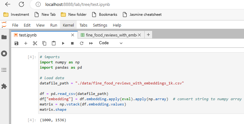
전체 소스코드는 아래와 같습니다.
# imports
import numpy as np
import pandas as pd
# load data
datafile_path = "./data/fine_food_reviews_with_embeddings_1k.csv"
df = pd.read_csv(datafile_path)
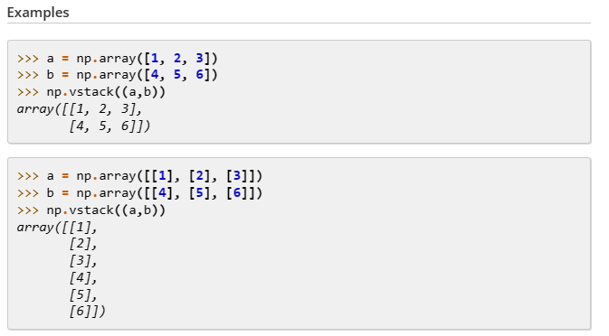
df["embedding"] = df.embedding.apply(eval).apply(np.array) # convert string to numpy array
matrix = np.vstack(df.embedding.values)
matrix.shape
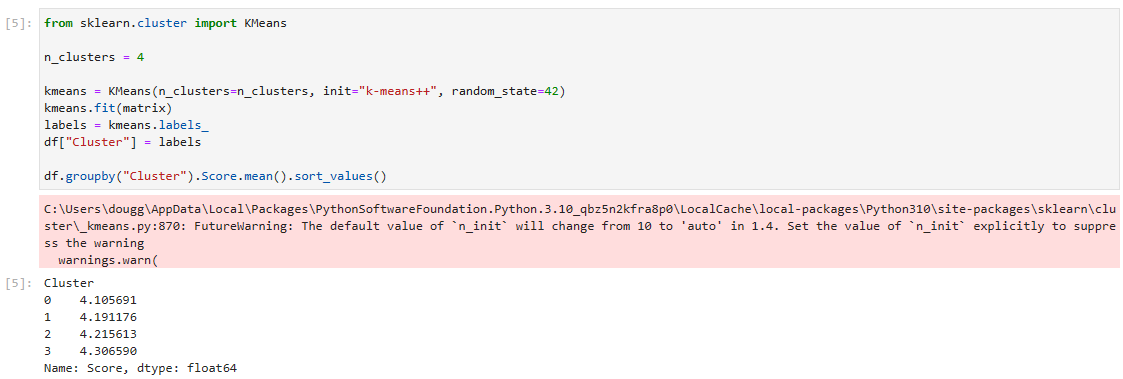
from sklearn.cluster import KMeans
n_clusters = 4
kmeans = KMeans(n_clusters=n_clusters, init="k-means++", random_state=42)
kmeans.fit(matrix)
labels = kmeans.labels_
df["Cluster"] = labels
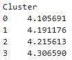
df.groupby("Cluster").Score.mean().sort_values()
from sklearn.manifold import TSNE
import matplotlib
import matplotlib.pyplot as plt
tsne = TSNE(n_components=2, perplexity=15, random_state=42, init="random", learning_rate=200)
vis_dims2 = tsne.fit_transform(matrix)
x = [x for x, y in vis_dims2]
y = [y for x, y in vis_dims2]
for category, color in enumerate(["purple", "green", "red", "blue"]):
xs = np.array(x)[df.Cluster == category]
ys = np.array(y)[df.Cluster == category]
plt.scatter(xs, ys, color=color, alpha=0.3)
avg_x = xs.mean()
avg_y = ys.mean()
plt.scatter(avg_x, avg_y, marker="x", color=color, s=100)
plt.title("Clusters identified visualized in language 2d using t-SNE")
import openai
def open_file(filepath):
with open(filepath, 'r', encoding='utf-8') as infile:
return infile.read()
openai.api_key = open_file('openaiapikey.txt')
# Reading a review which belong to each group.
rev_per_cluster = 5
for i in range(n_clusters):
print(f"Cluster {i} Theme:", end=" ")
reviews = "\n".join(
df[df.Cluster == i]
.combined.str.replace("Title: ", "")
.str.replace("\n\nContent: ", ": ")
.sample(rev_per_cluster, random_state=42)
.values
)
response = openai.Completion.create(
engine="text-ada-001", #"text-davinci-003",
prompt=f'What do the following customer reviews have in common?\n\nCustomer reviews:\n"""\n{reviews}\n"""\n\nTheme:',
temperature=0,
max_tokens=64,
top_p=1,
frequency_penalty=0,
presence_penalty=0,
)
print(response["choices"][0]["text"].replace("\n", ""))
sample_cluster_rows = df[df.Cluster == i].sample(rev_per_cluster, random_state=42)
for j in range(rev_per_cluster):
print(sample_cluster_rows.Score.values[j], end=", ")
print(sample_cluster_rows.Summary.values[j], end=": ")
print(sample_cluster_rows.Text.str[:70].values[j])
이 예제의 training data는 [text_1, text_2, label] 형식 입니다.
두 쌍이 유사하면 레이블은 +1 이고 유사하지 않으면 -1 입니다.
output은 임베딩을 multiply 하는데 사용할 수 있는 matrix 입니다.
임베딩 multiplication을 통해서 좀 더 성능이 좋은 custom embedding을 얻을 수 있습니다.
그 다음 예제는 SNLI corpus에서 가지고 온 1000개의 sentence pair들을 사용합니다. 이 두 쌍은 논리적으로 연관돼 있는데 한 문장이 다른 문장을 암시하는 식 입니다. 논리적으로 연관 돼 있으면 레이블이 positive 입니다. 논리적으로 연관이 별로 없어 보이는 쌍은 레이블이 negative 가 됩니다.
그리고 clustering을 사용하는 경우에는 같은 클러스터 내의 텍스트 들로부터 한 쌍을 만듦으로서 positive 한 것을 생성할 수 있습니다. 그리고 다른 클러스터의 문장들로 쌍을 이루어서 negative를 생성할 수 있습니다.
다른 데이터 세트를 사용하면 100개 미만의 training example들 만으로도 좋은 성능 개선을 이루는 것을 볼 수 있었습니다. 물론 더 많은 예제를 사용하면 더 좋아지겠죠.
이제 소스 코드로 들어가 보겠습니다.
0. Imports
# imports
from typing import List, Tuple # for type hints
import numpy as np # for manipulating arrays
import pandas as pd # for manipulating data in dataframes
import pickle # for saving the embeddings cache
import plotly.express as px # for plots
import random # for generating run IDs
from sklearn.model_selection import train_test_split # for splitting train & test data
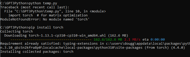
import torch # for matrix optimization
from openai.embeddings_utils import get_embedding, cosine_similarity # for embeddings
# input parameters
embedding_cache_path = "data/snli_embedding_cache.pkl" # embeddings will be saved/loaded here
default_embedding_engine = "babbage-similarity" # choice of: ada, babbage, curie, davinci
num_pairs_to_embed = 1000 # 1000 is arbitrary - I've gotten it to work with as little as ~100
local_dataset_path = "data/snli_1.0_train_2k.csv" # download from: https://nlp.stanford.edu/projects/snli/
def process_input_data(df: pd.DataFrame) -> pd.DataFrame:
# you can customize this to preprocess your own dataset
# output should be a dataframe with 3 columns: text_1, text_2, label (1 for similar, -1 for dissimilar)
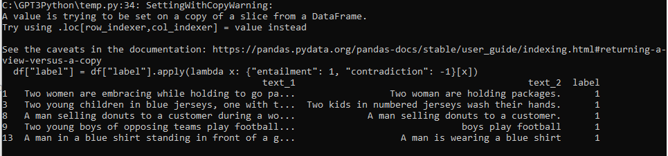
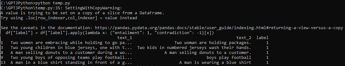
df["label"] = df["gold_label"]
df = df[df["label"].isin(["entailment"])]
df["label"] = df["label"].apply(lambda x: {"entailment": 1, "contradiction": -1}[x])
df = df.rename(columns={"sentence1": "text_1", "sentence2": "text_2"})
df = df[["text_1", "text_2", "label"]]
df = df.head(num_pairs_to_embed)
return df
여기서 하는 일은 cache 에 있는 데이터를 저장할 pkl 파일을 정하고 사용할 openai 모델을 정했습니다.
그리고 num_pairs_to_embed 변수에 1000을 할당했고 소스 데이터를 local_dataset_path 에 할당했습니다.
다음에 process_input_data() 함수가 나오는데요.
pandas 의 DataFrame 형식의 입력값을 받아서 처리한 다음에 다시 DataFrame형식으로 반환합니다.
대개 컬럼 이름들을 바꾸는 거네요.
그리고 DataFrame의 데이터를 1000 (num_pairs_to_embed) 개만 추려서 return 합니다.
2. Load and process input data
# load data
df = pd.read_csv(local_dataset_path)

# process input data
df = process_input_data(df)  # this demonstrates training data containing only positives

# view data
df.head()
이제 파일을 열고 위에 만들었던 함수를 통해 처리한 다음 상위 5개를 출력합니다.
df.head() 는 디폴트로 5개를 출력합니다. head() 안에 숫자를 넣으면 그 숫자만큼 출력합니다.
이걸 출력하면 이렇게 됩니다.
3. Split data into training test sets
synethetic negatives나 synethetic positives를 생성하기 전에 데이터를 training과 test sets 들로 구분하는 것은 아주 중요합니다.
training data의 text 문자열이 test data에 표시되는 것을 원하지 않을 겁니다.
contamination이 있는 경우 실제 production 보다 test metrics가 더 좋아 보일 수 있습니다.
# split data into train and test sets
test_fraction = 0.5  # 0.5 is fairly arbitrary
random_seed = 123  # random seed is arbitrary, but is helpful in reproducibility
train_df, test_df = train_test_split(
    df, test_size=test_fraction, stratify=df["label"], random_state=random_seed
)
train_df.loc[:, "dataset"] = "train"
test_df.loc[:, "dataset"] = "test"
여기에서는 sklearn.model_selection 모듈의 train_test_split() 함수를 사용해서 데이터를 training test sets로 분리 합니다.
4. Generate synthetic negatives
다음은 use case에 맞도록 수정해야 할 필요가 있을 수 있는 코드 입니다.
positives와 negarives 가 있는 데이터를 가지고 있을 경우 건너뛰어도 됩니다.
근데 만약 positives 한 데이터만 가지고 있다면 이 코드를 사용해야 할 것입니다.
이 코드 블록은 negatives 만 생성할 것입니다.
만약 여러분이 multiclass data를 가지고 있다면 여러분은 positives와 negatives 모두를 생성하기를 원할 겁니다.
positives는 레이블들을 공유하는 텍스트로 된 쌍이 될 수 있고 negatives는 레이블을 공유하지 않는 텍스트로 된 쌍이 될 수 있습니다.
최종 결과물은 text pair로 된 DataFrame이 될 것입니다. 각 쌍은 -1이나 1이 될 것입니다.
# generate negatives
def dataframe_of_negatives(dataframe_of_positives: pd.DataFrame) -> pd.DataFrame:
    """Return dataframe of negative pairs made by combining elements of positive pairs."""
    texts = set(dataframe_of_positives["text_1"].values) | set(
        dataframe_of_positives["text_2"].values
    )
    all_pairs = {(t1, t2) for t1 in texts for t2 in texts if t1 < t2}
    positive_pairs = set(
        tuple(text_pair)
        for text_pair in dataframe_of_positives[["text_1", "text_2"]].values
    )
    negative_pairs = all_pairs - positive_pairs
    df_of_negatives = pd.DataFrame(list(negative_pairs), columns=["text_1", "text_2"])
    df_of_negatives["label"] = -1
    return df_of_negatives
negatives_per_positive = (
    1  # it will work at higher values too, but more data will be slower
)
# generate negatives for training dataset
train_df_negatives = dataframe_of_negatives(train_df)
train_df_negatives["dataset"] = "train"
# generate negatives for test dataset
test_df_negatives = dataframe_of_negatives(test_df)
test_df_negatives["dataset"] = "test"
# sample negatives and combine with positives
train_df = pd.concat(
    [
        train_df,
        train_df_negatives.sample(
            n=len(train_df) * negatives_per_positive, random_state=random_seed
        ),
    ]
)
test_df = pd.concat(
    [
        test_df,
        test_df_negatives.sample(
            n=len(test_df) * negatives_per_positive, random_state=random_seed
        ),
    ]
)

df = pd.concat([train_df, test_df])
5. Calculate embeddings and cosine similarities
아래 코드 블럭에서는 임베딩을 저장하기 위한 캐시를 생성합니다.
이렇게 저장함으로서 다시 임베딩을 얻기 위해 openai api를 호출하면서 비용을 지불하지 않아도 됩니다.
# establish a cache of embeddings to avoid recomputing
# cache is a dict of tuples (text, engine) -> embedding
try:
with open(embedding_cache_path, "rb") as f:
embedding_cache = pickle.load(f)
except FileNotFoundError:
precomputed_embedding_cache_path = "https://cdn.openai.com/API/examples/data/snli_embedding_cache.pkl"
embedding_cache = pd.read_pickle(precomputed_embedding_cache_path)
# this function will get embeddings from the cache and save them there afterward
def get_embedding_with_cache(
text: str,
engine: str = default_embedding_engine,
embedding_cache: dict = embedding_cache,
embedding_cache_path: str = embedding_cache_path,
) -> list:
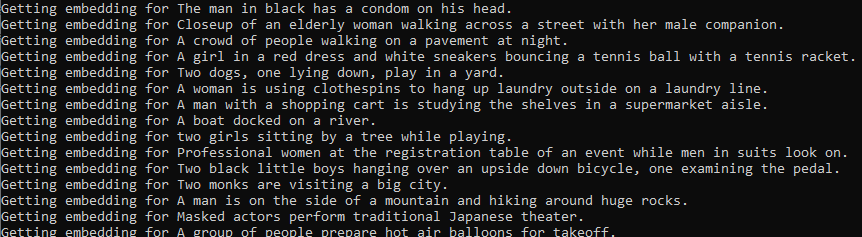
print(f"Getting embedding for {text}")
if (text, engine) not in embedding_cache.keys():
# if not in cache, call API to get embedding
embedding_cache[(text, engine)] = get_embedding(text, engine)
# save embeddings cache to disk after each update
with open(embedding_cache_path, "wb") as embedding_cache_file:
pickle.dump(embedding_cache, embedding_cache_file)
return embedding_cache[(text, engine)]
# create column of embeddings
for column in ["text_1", "text_2"]:
df[f"{column}_embedding"] = df[column].apply(get_embedding_with_cache)
# create column of cosine similarity between embeddings
df["cosine_similarity"] = df.apply(
lambda row: cosine_similarity(row["text_1_embedding"], row["text_2_embedding"]),
axis=1,
)
6. Plot distribution of cosine similarity
이 예제에서는 cosine similarity를 사용하여 텍스트의 유사성을 측정합니다. openai 측의 경험상 대부분의 distance functions (L1, L2, cosine similarity)들은 모두 동일하게 작동한다고 합니다. 임베딩 값은 length 가 1로 정규화 되어 있기 때문에 임베딩에서 cosine similarity는 python의 numpy.dot() 과 동일한 결과를 내 놓습니다.
그래프들은 유사한 쌍과 유사하지 않은 쌍에 대한 cosine similarity 분포 사이에 겹치는 정도를 보여 줍니다. 겹치는 부분이 많다면 다른 유사한 쌍보다 cosine similarity가 크고 유사하지 않은 쌍이 많다는 의미 입니다.
계산의 정확도는 cosine similarity의 특정 임계치인 X 보다 크면 similar (1)을 예측하고 그렇치 않으면 dissimilar (0)을 예측합니다.
# calculate accuracy (and its standard error) of predicting label=1 if similarity>x
# x is optimized by sweeping from -1 to 1 in steps of 0.01
def accuracy_and_se(cosine_similarity: float, labeled_similarity: int) -> Tuple[float]:
accuracies = []
for threshold_thousandths in range(-1000, 1000, 1):
threshold = threshold_thousandths / 1000
total = 0
correct = 0
for cs, ls in zip(cosine_similarity, labeled_similarity):
total += 1
if cs > threshold:
prediction = 1
else:
prediction = -1
if prediction == ls:
correct += 1
accuracy = correct / total
accuracies.append(accuracy)
a = max(accuracies)
n = len(cosine_similarity)
standard_error = (a * (1 - a) / n) ** 0.5 # standard error of binomial
return a, standard_error
# check that training and test sets are balanced
px.histogram(
df,
x="cosine_similarity",
color="label",
barmode="overlay",
width=500,
facet_row="dataset",
).show()
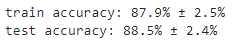
for dataset in ["train", "test"]:
data = df[df["dataset"] == dataset]
a, se = accuracy_and_se(data["cosine_similarity"], data["label"])
print(f"{dataset} accuracy: {a:0.1%} ± {1.96 * se:0.1%}")
여기까지 작성한 코드를 실행 해 봤습니다.
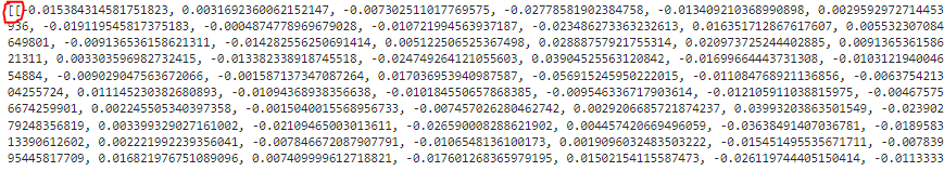
처음엔 아래 내용을 출력하더니......
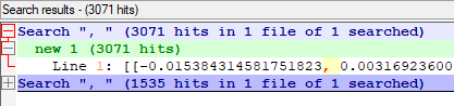
그 다음은 아래와 같은 형식으로 한도 끝도 없이 출력 하더라구요.
문서에 총 1만줄이 있던데 한줄 한줄 다 처리하느라 시간이 굉장히 많이 걸릴 것 같습니다.
전 3179 줄까지 출력한 후 시간이 너무 걸려서 강제로 중단 했습니다.
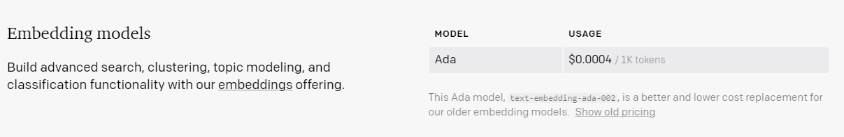
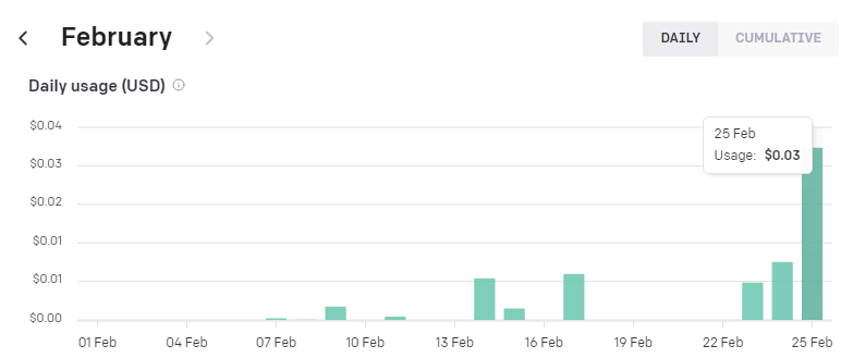
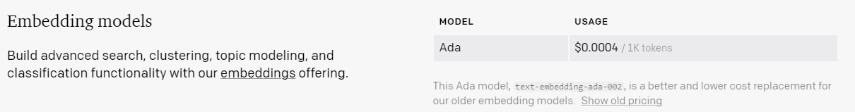
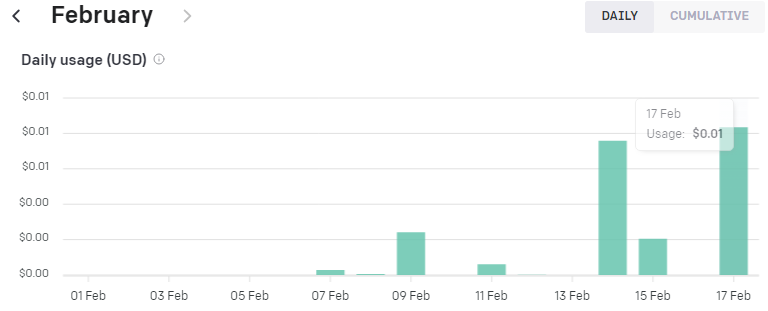
저는 text-embedding-ada-002 모델을 사용했습니다.
1천개의 토큰당 0.0004불이 과금 되는데 여기까지 저는 0.01불 즉 1센트가 과금 됐습니다.
그러면 0.01 / 0.0004 를 하니까 2만 5천 토큰 정도 사용 했나 보네요.
1만줄을 전부 다 하면 한 5센트 이내로 부과 되겠네요.
하여간 시간도 많이 걸리고 과금도 비교적 많이 되니 실행은 마지막에 딱 한번만 해 보기로 하겠습니다.
예제 상에는 6 Plot distribution of cosine similarity 에 있는 코드를 실행하면 아래와 같이 나온다고 합니다.
7. Optimize the matrix using the training data provided
def optimize_matrix(
modified_embedding_length: int = 2048, # in my brief experimentation, bigger was better (2048 is length of babbage encoding)
batch_size: int = 100,
max_epochs: int = 100,
learning_rate: float = 100.0, # seemed to work best when similar to batch size - feel free to try a range of values
dropout_fraction: float = 0.0, # in my testing, dropout helped by a couple percentage points (definitely not necessary)
df: pd.DataFrame = df,
print_progress: bool = True,
save_results: bool = True,
) -> torch.tensor:
"""Return matrix optimized to minimize loss on training data."""
run_id = random.randint(0, 2 ** 31 - 1) # (range is arbitrary)
# convert from dataframe to torch tensors
# e is for embedding, s for similarity label
def tensors_from_dataframe(
df: pd.DataFrame,
embedding_column_1: str,
embedding_column_2: str,
similarity_label_column: str,
) -> Tuple[torch.tensor]:
e1 = np.stack(np.array(df[embedding_column_1].values))
e2 = np.stack(np.array(df[embedding_column_2].values))
s = np.stack(np.array(df[similarity_label_column].astype("float").values))
e1 = torch.from_numpy(e1).float()
e2 = torch.from_numpy(e2).float()
s = torch.from_numpy(s).float()
return e1, e2, s
e1_train, e2_train, s_train = tensors_from_dataframe(
df[df["dataset"] == "train"], "text_1_embedding", "text_2_embedding", "label"
)
e1_test, e2_test, s_test = tensors_from_dataframe(
df[df["dataset"] == "train"], "text_1_embedding", "text_2_embedding", "label"
)
# create dataset and loader
dataset = torch.utils.data.TensorDataset(e1_train, e2_train, s_train)
train_loader = torch.utils.data.DataLoader(
dataset, batch_size=batch_size, shuffle=True
)
# define model (similarity of projected embeddings)
def model(embedding_1, embedding_2, matrix, dropout_fraction=dropout_fraction):
e1 = torch.nn.functional.dropout(embedding_1, p=dropout_fraction)
e2 = torch.nn.functional.dropout(embedding_2, p=dropout_fraction)
modified_embedding_1 = e1 @ matrix # @ is matrix multiplication
modified_embedding_2 = e2 @ matrix
similarity = torch.nn.functional.cosine_similarity(
modified_embedding_1, modified_embedding_2
)
return similarity
# define loss function to minimize
def mse_loss(predictions, targets):
difference = predictions - targets
return torch.sum(difference * difference) / difference.numel()
# initialize projection matrix
embedding_length = len(df["text_1_embedding"].values[0])
matrix = torch.randn(
embedding_length, modified_embedding_length, requires_grad=True
)
epochs, types, losses, accuracies, matrices = [], [], [], [], []
for epoch in range(1, 1 + max_epochs):
# iterate through training dataloader
for a, b, actual_similarity in train_loader:
# generate prediction
predicted_similarity = model(a, b, matrix)
# get loss and perform backpropagation
loss = mse_loss(predicted_similarity, actual_similarity)
loss.backward()
# update the weights
with torch.no_grad():
matrix -= matrix.grad * learning_rate
# set gradients to zero
matrix.grad.zero_()
# calculate test loss
test_predictions = model(e1_test, e2_test, matrix)
test_loss = mse_loss(test_predictions, s_test)
# compute custom embeddings and new cosine similarities
apply_matrix_to_embeddings_dataframe(matrix, df)
# calculate test accuracy
for dataset in ["train", "test"]:
data = df[df["dataset"] == dataset]
a, se = accuracy_and_se(data["cosine_similarity_custom"], data["label"])
# record results of each epoch
epochs.append(epoch)
types.append(dataset)
losses.append(loss.item() if dataset == "train" else test_loss.item())
accuracies.append(a)
matrices.append(matrix.detach().numpy())
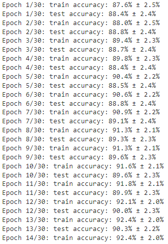
# optionally print accuracies
if print_progress is True:
print(
f"Epoch {epoch}/{max_epochs}: {dataset} accuracy: {a:0.1%} ± {1.96 * se:0.1%}"
)
data = pd.DataFrame(
{"epoch": epochs, "type": types, "loss": losses, "accuracy": accuracies}
)
data["run_id"] = run_id
data["modified_embedding_length"] = modified_embedding_length
data["batch_size"] = batch_size
data["max_epochs"] = max_epochs
data["learning_rate"] = learning_rate
data["dropout_fraction"] = dropout_fraction
data[
"matrix"
] = matrices # saving every single matrix can get big; feel free to delete/change
if save_results is True:
data.to_csv(f"{run_id}_optimization_results.csv", index=False)
return data
# example hyperparameter search
# I recommend starting with max_epochs=10 while initially exploring
results = []
max_epochs = 30
dropout_fraction = 0.2
for batch_size, learning_rate in [(10, 10), (100, 100), (1000, 1000)]:
result = optimize_matrix(
batch_size=batch_size,
learning_rate=learning_rate,
max_epochs=max_epochs,
dropout_fraction=dropout_fraction,
save_results=False,
)
results.append(result)
runs_df = pd.concat(results)
# plot training loss and test loss over time
px.line(
runs_df,
line_group="run_id",
x="epoch",
y="loss",
color="type",
hover_data=["batch_size", "learning_rate", "dropout_fraction"],
facet_row="learning_rate",
facet_col="batch_size",
width=500,
).show()
# plot accuracy over time
px.line(
runs_df,
line_group="run_id",
x="epoch",
y="accuracy",
color="type",
hover_data=["batch_size", "learning_rate", "dropout_fraction"],
facet_row="learning_rate",
facet_col="batch_size",
width=500,
).show()
이 부분은 7. Optimize the matrix using the training data provided 부분의 소스코드들 입니다.
embedding_multiplied_by_matrix() 함수는 임베딩 값과 matrix 값을 받아서 처리한 다음에 np.array 형식의 결과값을 반환합니다.
그 다음 함수는 apply_matrix_to_embeddings_dataframe() 함수로 기존의 임베딩 값과 새로운 cosine similarities 값으로 계산을 하는 일을 합니다. 여기에서 위의 함수인 embedding_multiplied_by_matrix() 함수를 호출한 후 그 결과 값을 받아서 처리합니다.
그 다음에도 여러 함수들이 있는데 따로 설명을 하면 너무 길어질 것 같네요.
각자 보면서 분석을 해야 할 것 같습니다.
여기까지 실행하면 아래와 같은 결과값을 볼 수 있습니다.
8. Plot the before & after, showing the results of the best matrix found during training
matrix 가 좋을 수록 similar pairs 와 dissimilar pairs를 더 명확하게 구분 할 수 있습니다.
# apply result of best run to original data
best_run = runs_df.sort_values(by="accuracy", ascending=False).iloc[0]
best_matrix = best_run["matrix"]
apply_matrix_to_embeddings_dataframe(best_matrix, df)
runs_df 는 위에서 정의한 df 변수 이름이고 그 다음의 sort_values() 는 pandas의 함수입니다.
그리고 이 정렬된 matrix 값을 7번에서 만든 apply_matrix_to_embeddings_dataframe() 에서 처리하도록 합니다.
# plot similarity distribution BEFORE customization
px.histogram(
df,
x="cosine_similarity",
color="label",
barmode="overlay",
width=500,
facet_row="dataset",
).show()
test_df = df[df["dataset"] == "test"]
a, se = accuracy_and_se(test_df["cosine_similarity"], test_df["label"])
print(f"Test accuracy: {a:0.1%} ± {1.96 * se:0.1%}")
# plot similarity distribution AFTER customization
px.histogram(
df,
x="cosine_similarity_custom",
color="label",
barmode="overlay",
width=500,
facet_row="dataset",
).show()
a, se = accuracy_and_se(test_df["cosine_similarity_custom"], test_df["label"])
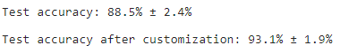
print(f"Test accuracy after customization: {a:0.1%} ± {1.96 * se:0.1%}")
여기서 이용한 함수는 6번에서 만든 accuracy_and_se() 함수 입니다. 정확도를 계산하는 함수였습니다.
여기서는 customization이 되기 전의 데이터인 cosine_similarity와 customization이 된 이후의 데이터인 cosine_similarrity_custom에 대해 accuracy_and_se() 함수로 정확도를 계산 한 값을 비교할 수 있도록 해 줍니다.
보시는 바와 같이 커스터마이징을 한 데이터가 정확도가 훨씬 높습니다.
best_matrix # this is what you can multiply your embeddings by
이렇게 해서 얻은 best_matrix 를 가지고 사용하면 훨씬 더 좋은 결과를 얻을 수 있습니다.
# imports
from typing import List, Tuple # for type hints
import openai
import numpy as np # for manipulating arrays
import pandas as pd # for manipulating data in dataframes
import pickle # for saving the embeddings cache
import plotly.express as px # for plots
import random # for generating run IDs
from sklearn.model_selection import train_test_split # for splitting train & test data
import torch # for matrix optimization
from openai.embeddings_utils import get_embedding, cosine_similarity # for embeddings
def open_file(filepath):
with open(filepath, 'r', encoding='utf-8') as infile:
return infile.read()
openai.api_key = open_file('openaiapikey.txt')
# input parameters
embedding_cache_path = "data/snli_embedding_cache.pkl" # embeddings will be saved/loaded here
#default_embedding_engine = "babbage-similarity" # choice of: ada, babbage, curie, davinci
#default_embedding_engine = "ada-similarity"
default_embedding_engine = "text-embedding-ada-002"
num_pairs_to_embed = 1000 # 1000 is arbitrary - I've gotten it to work with as little as ~100
local_dataset_path = "data/snli_1.0_train_2k.csv" # download from: https://nlp.stanford.edu/projects/snli/
def process_input_data(df: pd.DataFrame) -> pd.DataFrame:
# you can customize this to preprocess your own dataset
# output should be a dataframe with 3 columns: text_1, text_2, label (1 for similar, -1 for dissimilar)
df["label"] = df["gold_label"]
df = df[df["label"].isin(["entailment"])]
df["label"] = df["label"].apply(lambda x: {"entailment": 1, "contradiction": -1}[x])
df = df.rename(columns={"sentence1": "text_1", "sentence2": "text_2"})
df = df[["text_1", "text_2", "label"]]
df = df.head(num_pairs_to_embed)
return df
# load data
df = pd.read_csv(local_dataset_path)
# process input data
df = process_input_data(df) # this demonstrates training data containing only positives
# view data
result = df.head()
print(result)
# split data into train and test sets
test_fraction = 0.5 # 0.5 is fairly arbitrary
random_seed = 123 # random seed is arbitrary, but is helpful in reproducibility
train_df, test_df = train_test_split(
df, test_size=test_fraction, stratify=df["label"], random_state=random_seed
)
train_df.loc[:, "dataset"] = "train"
test_df.loc[:, "dataset"] = "test"
# generate negatives
def dataframe_of_negatives(dataframe_of_positives: pd.DataFrame) -> pd.DataFrame:
"""Return dataframe of negative pairs made by combining elements of positive pairs."""
texts = set(dataframe_of_positives["text_1"].values) | set(
dataframe_of_positives["text_2"].values
)
all_pairs = {(t1, t2) for t1 in texts for t2 in texts if t1 < t2}
positive_pairs = set(
tuple(text_pair)
for text_pair in dataframe_of_positives[["text_1", "text_2"]].values
)
negative_pairs = all_pairs - positive_pairs
df_of_negatives = pd.DataFrame(list(negative_pairs), columns=["text_1", "text_2"])
df_of_negatives["label"] = -1
return df_of_negatives
negatives_per_positive = (
1 # it will work at higher values too, but more data will be slower
)
# generate negatives for training dataset
train_df_negatives = dataframe_of_negatives(train_df)
train_df_negatives["dataset"] = "train"
# generate negatives for test dataset
test_df_negatives = dataframe_of_negatives(test_df)
test_df_negatives["dataset"] = "test"
# sample negatives and combine with positives
train_df = pd.concat(
[
train_df,
train_df_negatives.sample(
n=len(train_df) * negatives_per_positive, random_state=random_seed
),
]
)
test_df = pd.concat(
[
test_df,
test_df_negatives.sample(
n=len(test_df) * negatives_per_positive, random_state=random_seed
),
]
)
df = pd.concat([train_df, test_df])
# establish a cache of embeddings to avoid recomputing
# cache is a dict of tuples (text, engine) -> embedding
try:
with open(embedding_cache_path, "rb") as f:
embedding_cache = pickle.load(f)
except FileNotFoundError:
precomputed_embedding_cache_path = "https://cdn.openai.com/API/examples/data/snli_embedding_cache.pkl"
embedding_cache = pd.read_pickle(precomputed_embedding_cache_path)
# this function will get embeddings from the cache and save them there afterward
def get_embedding_with_cache(
text: str,
engine: str = default_embedding_engine,
embedding_cache: dict = embedding_cache,
embedding_cache_path: str = embedding_cache_path,
) -> list:
print(f"Getting embedding for {text}")
if (text, engine) not in embedding_cache.keys():
# if not in cache, call API to get embedding
embedding_cache[(text, engine)] = get_embedding(text, engine)
# save embeddings cache to disk after each update
with open(embedding_cache_path, "wb") as embedding_cache_file:
pickle.dump(embedding_cache, embedding_cache_file)
return embedding_cache[(text, engine)]
# create column of embeddings
for column in ["text_1", "text_2"]:
df[f"{column}_embedding"] = df[column].apply(get_embedding_with_cache)
# create column of cosine similarity between embeddings
df["cosine_similarity"] = df.apply(
lambda row: cosine_similarity(row["text_1_embedding"], row["text_2_embedding"]),
axis=1,
)
# calculate accuracy (and its standard error) of predicting label=1 if similarity>x
# x is optimized by sweeping from -1 to 1 in steps of 0.01
def accuracy_and_se(cosine_similarity: float, labeled_similarity: int) -> Tuple[float]:
accuracies = []
for threshold_thousandths in range(-1000, 1000, 1):
threshold = threshold_thousandths / 1000
total = 0
correct = 0
for cs, ls in zip(cosine_similarity, labeled_similarity):
total += 1
if cs > threshold:
prediction = 1
else:
prediction = -1
if prediction == ls:
correct += 1
accuracy = correct / total
accuracies.append(accuracy)
a = max(accuracies)
n = len(cosine_similarity)
standard_error = (a * (1 - a) / n) ** 0.5 # standard error of binomial
return a, standard_error
# check that training and test sets are balanced
px.histogram(
df,
x="cosine_similarity",
color="label",
barmode="overlay",
width=500,
facet_row="dataset",
).show()
for dataset in ["train", "test"]:
data = df[df["dataset"] == dataset]
a, se = accuracy_and_se(data["cosine_similarity"], data["label"])
print(f"{dataset} accuracy: {a:0.1%} ± {1.96 * se:0.1%}")
def embedding_multiplied_by_matrix(
    embedding: List[float], matrix: torch.tensor
) -> np.array:
    embedding_tensor = torch.tensor(embedding).float()
    modified_embedding = embedding_tensor @ matrix
    modified_embedding = modified_embedding.detach().numpy()
    return modified_embedding


# compute custom embeddings and new cosine similarities
def apply_matrix_to_embeddings_dataframe(matrix: torch.tensor, df: pd.DataFrame):
    for column in ["text_1_embedding", "text_2_embedding"]:
        df[f"{column}_custom"] = df[column].apply(
            lambda x: embedding_multiplied_by_matrix(x, matrix)
        )
    df["cosine_similarity_custom"] = df.apply(
        lambda row: cosine_similarity(
            row["text_1_embedding_custom"], row["text_2_embedding_custom"]
        ),
        axis=1,
    )
def optimize_matrix(
    modified_embedding_length: int = 2048,  # in my brief experimentation, bigger was better (2048 is length of babbage encoding)
    batch_size: int = 100,
    max_epochs: int = 100,
    learning_rate: float = 100.0,  # seemed to work best when similar to batch size - feel free to try a range of values
    dropout_fraction: float = 0.0,  # in my testing, dropout helped by a couple percentage points (definitely not necessary)
    df: pd.DataFrame = df,
    print_progress: bool = True,
    save_results: bool = True,
) -> torch.tensor:
    """Return matrix optimized to minimize loss on training data."""
    run_id = random.randint(0, 2 ** 31 - 1)  # (range is arbitrary)
    # convert from dataframe to torch tensors
    # e is for embedding, s for similarity label
    def tensors_from_dataframe(
        df: pd.DataFrame,
        embedding_column_1: str,
        embedding_column_2: str,
        similarity_label_column: str,
    ) -> Tuple[torch.tensor]:
        e1 = np.stack(np.array(df[embedding_column_1].values))
        e2 = np.stack(np.array(df[embedding_column_2].values))
        s = np.stack(np.array(df[similarity_label_column].astype("float").values))

        e1 = torch.from_numpy(e1).float()
        e2 = torch.from_numpy(e2).float()
        s = torch.from_numpy(s).float()

        return e1, e2, s

    e1_train, e2_train, s_train = tensors_from_dataframe(
        df[df["dataset"] == "train"], "text_1_embedding", "text_2_embedding", "label"
    )
    e1_test, e2_test, s_test = tensors_from_dataframe(
        df[df["dataset"] == "train"], "text_1_embedding", "text_2_embedding", "label"
    )

    # create dataset and loader
    dataset = torch.utils.data.TensorDataset(e1_train, e2_train, s_train)
    train_loader = torch.utils.data.DataLoader(
        dataset, batch_size=batch_size, shuffle=True
    )

    # define model (similarity of projected embeddings)
    def model(embedding_1, embedding_2, matrix, dropout_fraction=dropout_fraction):
        e1 = torch.nn.functional.dropout(embedding_1, p=dropout_fraction)
        e2 = torch.nn.functional.dropout(embedding_2, p=dropout_fraction)
        modified_embedding_1 = e1 @ matrix  # @ is matrix multiplication
        modified_embedding_2 = e2 @ matrix
        similarity = torch.nn.functional.cosine_similarity(
            modified_embedding_1, modified_embedding_2
        )
        return similarity

    # define loss function to minimize
    def mse_loss(predictions, targets):
        difference = predictions - targets
        return torch.sum(difference * difference) / difference.numel()

    # initialize projection matrix
    embedding_length = len(df["text_1_embedding"].values[0])
    matrix = torch.randn(
        embedding_length, modified_embedding_length, requires_grad=True
    )

    epochs, types, losses, accuracies, matrices = [], [], [], [], []
    for epoch in range(1, 1 + max_epochs):
        # iterate through training dataloader
        for a, b, actual_similarity in train_loader:
            # generate prediction
            predicted_similarity = model(a, b, matrix)
            # get loss and perform backpropagation
            loss = mse_loss(predicted_similarity, actual_similarity)
            loss.backward()
            # update the weights
            with torch.no_grad():
                matrix -= matrix.grad * learning_rate
                # set gradients to zero
                matrix.grad.zero_()
        # calculate test loss
        test_predictions = model(e1_test, e2_test, matrix)
        test_loss = mse_loss(test_predictions, s_test)

        # compute custom embeddings and new cosine similarities
        apply_matrix_to_embeddings_dataframe(matrix, df)

        # calculate test accuracy
        for dataset in ["train", "test"]:
            data = df[df["dataset"] == dataset]
            a, se = accuracy_and_se(data["cosine_similarity_custom"], data["label"])

            # record results of each epoch
            epochs.append(epoch)
            types.append(dataset)
            losses.append(loss.item() if dataset == "train" else test_loss.item())
            accuracies.append(a)
            matrices.append(matrix.detach().numpy())

            # optionally print accuracies
            if print_progress is True:
                print(
                    f"Epoch {epoch}/{max_epochs}: {dataset} accuracy: {a:0.1%} ± {1.96 * se:0.1%}"
                )

    data = pd.DataFrame(
        {"epoch": epochs, "type": types, "loss": losses, "accuracy": accuracies}
    )
    data["run_id"] = run_id
    data["modified_embedding_length"] = modified_embedding_length
    data["batch_size"] = batch_size
    data["max_epochs"] = max_epochs
    data["learning_rate"] = learning_rate
    data["dropout_fraction"] = dropout_fraction
    data[
        "matrix"
    ] = matrices  # saving every single matrix can get big; feel free to delete/change
    if save_results is True:
        data.to_csv(f"{run_id}_optimization_results.csv", index=False)

    return data
# example hyperparameter search
# I recommend starting with max_epochs=10 while initially exploring
results = []
max_epochs = 30
dropout_fraction = 0.2
for batch_size, learning_rate in [(10, 10), (100, 100), (1000, 1000)]:
    result = optimize_matrix(
        batch_size=batch_size,
        learning_rate=learning_rate,
        max_epochs=max_epochs,
        dropout_fraction=dropout_fraction,
        save_results=False,
    )
    results.append(result)
runs_df = pd.concat(results)

# plot training loss and test loss over time
px.line(
    runs_df,
    line_group="run_id",
    x="epoch",
    y="loss",
    color="type",
    hover_data=["batch_size", "learning_rate", "dropout_fraction"],
    facet_row="learning_rate",
    facet_col="batch_size",
    width=500,
).show()

# plot accuracy over time
px.line(
    runs_df,
    line_group="run_id",
    x="epoch",
    y="accuracy",
    color="type",
    hover_data=["batch_size", "learning_rate", "dropout_fraction"],
    facet_row="learning_rate",
    facet_col="batch_size",
    width=500,
).show()
# apply result of best run to original data
best_run = runs_df.sort_values(by="accuracy", ascending=False).iloc[0]
best_matrix = best_run["matrix"]
apply_matrix_to_embeddings_dataframe(best_matrix, df)
# plot similarity distribution BEFORE customization
px.histogram(
    df,
    x="cosine_similarity",
    color="label",
    barmode="overlay",
    width=500,
    facet_row="dataset",
).show()

test_df = df[df["dataset"] == "test"]
a, se = accuracy_and_se(test_df["cosine_similarity"], test_df["label"])
print(f"Test accuracy: {a:0.1%} ± {1.96 * se:0.1%}")

# plot similarity distribution AFTER customization
px.histogram(
    df,
    x="cosine_similarity_custom",
    color="label",
    barmode="overlay",
    width=500,
    facet_row="dataset",
).show()

a, se = accuracy_and_se(test_df["cosine_similarity_custom"], test_df["label"])
print(f"Test accuracy after customization: {a:0.1%} ± {1.96 * se:0.1%}")
best_matrix # this is what you can multiply your embeddings by
데이터 구조를 byte stream으로 변환하면 저장하거나 네트워크로 전송할 수 있습니다.
이런 것을 marshalling 이라고 하고 그 반대를 unmarshalling 이라고 합니다.
이런 작업을 할 수 있는 모듈은 아래 세가지가 있습니다.
marshal은 셋 중 가장 오래된 모듈이다. 이것은 주로 컴파일된 바이트코드 또는 인터프리터가 파이썬 모듈을 가져올 떄 얻는 .pyc 파일을 읽고 쓰기 위해 존재한다. 때문에 marshal로 객체를 직렬화할 수 있더라도, 이를 추천하지는 않는다.
json모듈은 셋 중 가장 최신의 모듈이다. 이를 통해 표준 JSON 파일로 작업을 할 수 있다. json 모듈을 통해 다양한 표준 파이썬 타입(bool, dict, int, float, list, string, tuple, None)을 직렬화, 역직렬화할 수 있다. json은 사람이 읽을 수 있고, 언어에 의존적이지 않다는 장점이 있다.
pickle모듈은 파이썬에서 객체를 직렬화 또는 역직렬화하는 또 다른 방식이다. json 모듈과는 다르게 객체를바이너리 포맷으로 직렬화한다. 이는 결과를 사람이 읽을 수 없다는 것을 의미한다. 그러나더 빠르고, 사용자 커스텀 객체 등더 다양한 파이썬 타입으로 동작할 수 있음을 의미한다.
bz2 를 csv 로 convert 시키는 온라인 툴에서 변환을 시도 했는데 너무 크기가 커서 실패 했습니다.
그래서 데이터소스가 없어서 이번 예제는 실행은 못 해 보고 소스만 분석하겠습니다.
위의 소스 코드는 데이터를 pandas의 read_csv() 로 읽어서 첫번째 5개만 df에 담는 역할을 합니다.
이런 결과를 얻을 수 있습니다.
# print the title, description, and label of each example
for idx, row in df.head(n_examples).iterrows():
print("")
print(f"Title: {row['title']}")
print(f"Description: {row['description']}")
print(f"Label: {row['label']}")
그 다음은 Title, Description, Lable 을 print 하는 부분 입니다.
여기까지 만들고 실행하면 아래 결과를 얻을 수 있습니다.
Title: World Briefings
Description: BRITAIN: BLAIR WARNS OF CLIMATE THREAT Prime Minister Tony Blair urged the international community to consider global warming a dire threat and agree on a plan of action to curb the quot;alarming quot; growth of greenhouse gases.
Label: World
Title: Nvidia Puts a Firewall on a Motherboard (PC World)
Description: PC World - Upcoming chip set will include built-in security features for your PC.
Label: Sci/Tech
Title: Olympic joy in Greek, Chinese press
Description: Newspapers in Greece reflect a mixture of exhilaration that the Athens Olympics proved successful, and relief that they passed off without any major setback.
Label: Sports
Title: U2 Can iPod with Pictures
Description: SAN JOSE, Calif. -- Apple Computer (Quote, Chart) unveiled a batch of new iPods, iTunes software and promos designed to keep it atop the heap of digital music players.
Label: Sci/Tech
Title: The Dream Factory
Description: Any product, any shape, any size -- manufactured on your desktop! The future is the fabricator. By Bruce Sterling from Wired magazine.
Label: Sci/Tech
여기까지 진행하면 아래와 같은 소스코드를 얻을 수 있을 겁니다.
# imports
import pandas as pd
import pickle
import openai
from openai.embeddings_utils import (
get_embedding,
distances_from_embeddings,
tsne_components_from_embeddings,
chart_from_components,
indices_of_nearest_neighbors_from_distances,
)
# constants
EMBEDDING_MODEL = "text-embedding-ada-002"
def open_file(filepath):
with open(filepath, 'r', encoding='utf-8') as infile:
return infile.read()
openai.api_key = open_file('openaiapikey.txt')
# load data (full dataset available at http://groups.di.unipi.it/~gulli/AG_corpus_of_news_articles.html)
dataset_path = "data/AG_news_samples.csv"
df = pd.read_csv(dataset_path)

# print dataframe
n_examples = 5
df.head(n_examples)
# print the title, description, and label of each example
for idx, row in df.head(n_examples).iterrows():
    print("")
    print(f"Title: {row['title']}")
    print(f"Description: {row['description']}")
    print(f"Label: {row['label']}")
3. Build cache to save embeddings
이 기사들에 대해 임베딩 값을 얻기 전에 임베딩을 값을 저장할 캐시를 세팅해 보겠습니다.
이렇게 얻은 임베딩을 저장해서 재 사용하면 이 값을 얻기 위해 openai api를 call 하지 않아도 되기 때문에 비용을 절감할 수 있습니다.
이 캐시는 dictionary로 (text, model) 의 tuples로 매핑되 있습니다.
이 캐시는 Python pickle 파일로 저장 될 것입니다.
# establish a cache of embeddings to avoid recomputing
# cache is a dict of tuples (text, model) -> embedding, saved as a pickle file
# set path to embedding cache
embedding_cache_path = "data/recommendations_embeddings_cache.pkl"
# load the cache if it exists, and save a copy to disk
try:
embedding_cache = pd.read_pickle(embedding_cache_path)
except FileNotFoundError:
embedding_cache = {}
with open(embedding_cache_path, "wb") as embedding_cache_file:
pickle.dump(embedding_cache, embedding_cache_file)
# define a function to retrieve embeddings from the cache if present, and otherwise request via the API
def embedding_from_string(
string: str,
model: str = EMBEDDING_MODEL,
embedding_cache=embedding_cache
) -> list:
"""Return embedding of given string, using a cache to avoid recomputing."""
if (string, model) not in embedding_cache.keys():
embedding_cache[(string, model)] = get_embedding(string, model)
with open(embedding_cache_path, "wb") as embedding_cache_file:
pickle.dump(embedding_cache, embedding_cache_file)
return embedding_cache[(string, model)]
처음에 저장될 위치와 pkl 파일 이름을 embedding_cache_path 변수에 담습니다.
다음은 이 cache가 있으면 카피를 저장하는 보분입니다.
pandas의 read_pickle() 함수를 통해 읽습니다. (embedding_cache에 담음)
이 파일을 오픈할 때 사용한 wb 는 파일을 binary format으로 오픈하고 쓰기 기능이 있다는 의미 입니다.
그 다음은 embedding_from_string() 함수 입니다.
입력값으로는 string과 openai의 모델명 그리고 embedding_cache를 받습니다.
출력은 리스트 형식입니다.
다음 if 문은 sriing과 model 이 embedding_cache.keys() 에 없다면 get_embedding()을 통해서 임베딩 값을 얻는 일을 합니다. 여기서도 파일은 바이너리 형태로 열고 쓰기 기능이 허락돼 있습니다.
pickle.dump()는 해당 내용을 파일에 저장할 때사용하는 pickle 모듈의 api 함수 입니다.
# as an example, take the first description from the dataset
example_string = df["description"].values[0]
print(f"\nExample string: {example_string}")
# print the first 10 dimensions of the embedding
example_embedding = embedding_from_string(example_string)
print(f"\nExample embedding: {example_embedding[:10]}...")
이 부분은 위에 작성한 스크립트가 잘 작동하는지 print 해 보는 겁니다.
여기까지 작성 한 것을 실행 하면 아래 출력을 얻을 수 있습니다.
4. Recommend similar articles based on embeddings
비슷한 기사를 찾기 위해서는 아래 3단계를 거쳐야 합니다.
1. 모든 기사의 description들에 대해 similarity 임베딩 값을 얻는다.
2. 소스 타이틀과 다른 모든 기사들간의 distance를 계산한다.
3. source title에 다른 기사들의 closest를 프린트 한다.
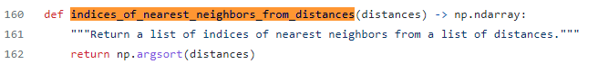
def print_recommendations_from_strings(
strings: list[str],
index_of_source_string: int,
k_nearest_neighbors: int = 1,
model=EMBEDDING_MODEL,
) -> list[int]:
"""Print out the k nearest neighbors of a given string."""
# get embeddings for all strings
embeddings = [embedding_from_string(string, model=model) for string in strings]
# get the embedding of the source string
query_embedding = embeddings[index_of_source_string]
# get distances between the source embedding and other embeddings (function from embeddings_utils.py)
distances = distances_from_embeddings(query_embedding, embeddings, distance_metric="cosine")
# get indices of nearest neighbors (function from embeddings_utils.py)
indices_of_nearest_neighbors = indices_of_nearest_neighbors_from_distances(distances)
# print out source string
query_string = strings[index_of_source_string]
print(f"Source string: {query_string}")
# print out its k nearest neighbors
k_counter = 0
for i in indices_of_nearest_neighbors:
# skip any strings that are identical matches to the starting string
if query_string == strings[i]:
continue
# stop after printing out k articles
if k_counter >= k_nearest_neighbors:
break
k_counter += 1
# print out the similar strings and their distances
print(
f"""
--- Recommendation #{k_counter} (nearest neighbor {k_counter} of {k_nearest_neighbors}) ---
String: {strings[i]}
Distance: {distances[i]:0.3f}"""
)
return indices_of_nearest_neighbors
이 소스 코드가 그 일을 합니다.
모든 string들에 대한 임베딩 값들을 받아서 distance를 구합니다. (distances_from_embeddings())
그리고 나서 가장 가까운 neighbor들을 구합니다. (indices_of_nearest_neighbors_from_distances())
그리고 query string을 print 합니다.
그리고 indices_of_nearest_neighbors 에 있는 요소들 만큼 for 루프를 돌리면서 Recommendation을 String, Distance 정보와 함께 print 합니다.
최종적으로 indices_of_nearest_neighbors를 return 합니다.
5. Example recommendations
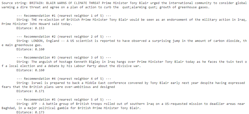
우선 Tony Blair에 대한 유사한 아티클들을 먼저 보죠.
article_descriptions = df["description"].tolist()
tony_blair_articles = print_recommendations_from_strings(
strings=article_descriptions, # let's base similarity off of the article description
index_of_source_string=0, # let's look at articles similar to the first one about Tony Blair
k_nearest_neighbors=5, # let's look at the 5 most similar articles
)
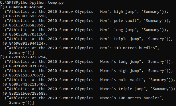
이렇게 하면 다음과 같은 정보를 얻을 수 있습니다.
첫 4개 기사에 토니 블레어가 언급 돼 있고 다섯번째에는 런던발 기후 변화에 대한 내용이 있습니다. 이것도 토니 블레어와 연관이 있다고 얘기할 수 있겠네요.
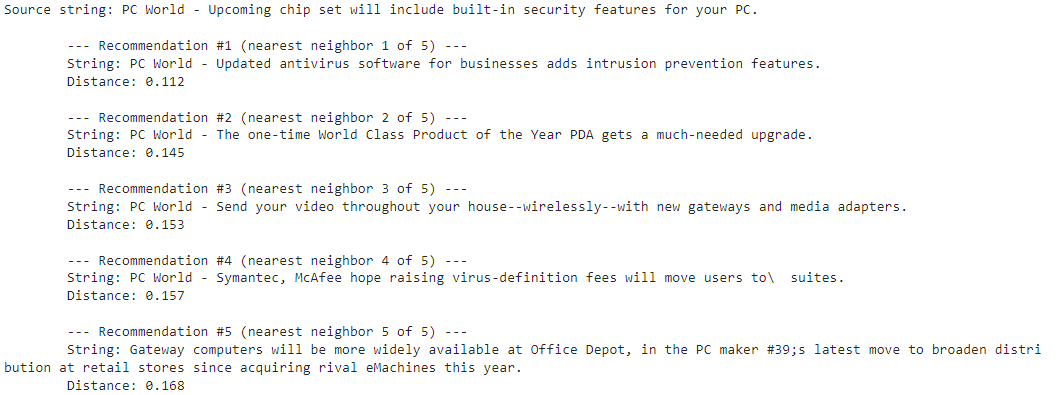
그러면 두번째 주제인 NVIDIA에 대한 결과물을 보겠습니다.
chipset_security_articles = print_recommendations_from_strings(
strings=article_descriptions, # let's base similarity off of the article description
index_of_source_string=1, # let's look at articles similar to the second one about a more secure chipset
k_nearest_neighbors=5, # let's look at the 5 most similar articles
)
결과를 보면 #1이 다른 결과물들 보다 가장 유사성이 큰 것을 볼 수 있습니다. (거리가 가깝다)
그 내용도 주어진 주제와 가장 가깝습니다.
Appendix: Using embeddings in more sophisticated recommenders
이 추천 시스템을 빌드하기 위한 좀 더 정교한 방법은 항목의 인기도, 사용자 클릭 데이터 같은 수많은 signal들을 가지고 machine learning 모델을 훈련 시키는 것입니다.
추천 시스템에서도 임베딩은 아주 유용하게 이용될 수 있습니다.
아직 기존의 유저 데이터가 없는 신제품에 대한 정보 같은 것들에 대해서 특히 이 임베딩은 잘 사용될 수 있습니다.
Appendix: Using embeddings to visualize similar articles
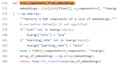
이 임베딩을 시각화 할 수도 있습니다. t-SNE 혹은 PCA와 같은 기술을 이용해서 임베딩을 2차원 또는 3차원 챠트로 만들 수 있습니다.
여기서는 t-SNE를 사용해서 모든 기사 설명을 시각화 해 봅니다.
(이와 관련된 결과물은 실행 때마다 조금씩 달라질 수 있습니다.)
# get embeddings for all article descriptions
embeddings = [embedding_from_string(string) for string in article_descriptions]
# compress the 2048-dimensional embeddings into 2 dimensions using t-SNE
tsne_components = tsne_components_from_embeddings(embeddings)
# get the article labels for coloring the chart
labels = df["label"].tolist()
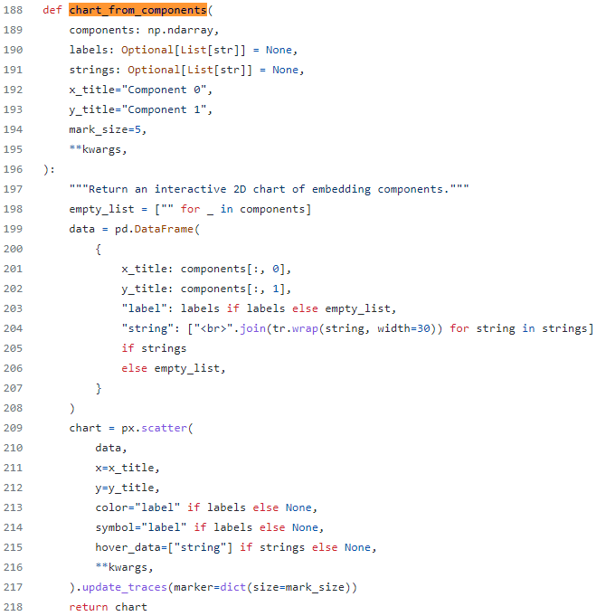
chart_from_components(
components=tsne_components,
labels=labels,
strings=article_descriptions,
width=600,
height=500,
title="t-SNE components of article descriptions",
)
다음은 source article, nearest neighbors 혹은 그 외 다른 것인지에 따라 다른 색으로 나타내 보는 코드 입니다.
# create labels for the recommended articles
def nearest_neighbor_labels(
list_of_indices: list[int],
k_nearest_neighbors: int = 5
) -> list[str]:
"""Return a list of labels to color the k nearest neighbors."""
labels = ["Other" for _ in list_of_indices]
source_index = list_of_indices[0]
labels[source_index] = "Source"
for i in range(k_nearest_neighbors):
nearest_neighbor_index = list_of_indices[i + 1]
labels[nearest_neighbor_index] = f"Nearest neighbor (top {k_nearest_neighbors})"
return labels
tony_blair_labels = nearest_neighbor_labels(tony_blair_articles, k_nearest_neighbors=5)
chipset_security_labels = nearest_neighbor_labels(chipset_security_articles, k_nearest_neighbors=5
)
# a 2D chart of nearest neighbors of the Tony Blair article
chart_from_components(
components=tsne_components,
labels=tony_blair_labels,
strings=article_descriptions,
width=600,
height=500,
title="Nearest neighbors of the Tony Blair article",
category_orders={"label": ["Other", "Nearest neighbor (top 5)", "Source"]},
)
# a 2D chart of nearest neighbors of the chipset security article
chart_from_components(
components=tsne_components,
labels=chipset_security_labels,
strings=article_descriptions,
width=600,
height=500,
title="Nearest neighbors of the chipset security article",
category_orders={"label": ["Other", "Nearest neighbor (top 5)", "Source"]},
)
이런 과정을 통해 결과를 시각화 하면 좀 더 다양한 정보들을 얻을 수 있습니다.
이번 예제는 여기서 사용된 소스 데이터를 구하지 못해서 직접 실행은 못해 봤네요.
다음에 소스데이터를 구할 기회가 생기면 한번 직접 실행 해 봐야 겠습니다.
이 예제를 전부 완성하면 아래와 같은 소스 코드가 될 것입니다.
# imports
import pandas as pd
import pickle
import openai

from openai.embeddings_utils import (
    get_embedding,
    distances_from_embeddings,
    tsne_components_from_embeddings,
    chart_from_components,
    indices_of_nearest_neighbors_from_distances,
)

# constants
EMBEDDING_MODEL = "text-embedding-ada-002"

def open_file(filepath):
    with open(filepath, 'r', encoding='utf-8') as infile:
        return infile.read()

openai.api_key = open_file('openaiapikey.txt')

# load data (full dataset available at http://groups.di.unipi.it/~gulli/AG_corpus_of_news_articles.html)
dataset_path = "data/AG_news_samples.csv"
df = pd.read_csv(dataset_path)

# print dataframe
n_examples = 5
df.head(n_examples)

# print the title, description, and label of each example
for idx, row in df.head(n_examples).iterrows():
    print("")
    print(f"Title: {row['title']}")
    print(f"Description: {row['description']}")
    print(f"Label: {row['label']}")
# establish a cache of embeddings to avoid recomputing
# cache is a dict of tuples (text, model) -> embedding, saved as a pickle file

# set path to embedding cache
embedding_cache_path = "data/recommendations_embeddings_cache.pkl"

# load the cache if it exists, and save a copy to disk
try:
    embedding_cache = pd.read_pickle(embedding_cache_path)
except FileNotFoundError:
    embedding_cache = {}
with open(embedding_cache_path, "wb") as embedding_cache_file:
    pickle.dump(embedding_cache, embedding_cache_file)

# define a function to retrieve embeddings from the cache if present, and otherwise request via the API
def embedding_from_string(
    string: str,
    model: str = EMBEDDING_MODEL,
    embedding_cache=embedding_cache
) -> list:
    """Return embedding of given string, using a cache to avoid recomputing."""
    if (string, model) not in embedding_cache.keys():
        embedding_cache[(string, model)] = get_embedding(string, model)
        with open(embedding_cache_path, "wb") as embedding_cache_file:
            pickle.dump(embedding_cache, embedding_cache_file)
    return embedding_cache[(string, model)]
# as an example, take the first description from the dataset
example_string = df["description"].values[0]
print(f"\nExample string: {example_string}")

# print the first 10 dimensions of the embedding
example_embedding = embedding_from_string(example_string)
print(f"\nExample embedding: {example_embedding[:10]}...")
def print_recommendations_from_strings(
    strings: list[str],
    index_of_source_string: int,
    k_nearest_neighbors: int = 1,
    model=EMBEDDING_MODEL,
) -> list[int]:
    """Print out the k nearest neighbors of a given string."""
    # get embeddings for all strings
    embeddings = [embedding_from_string(string, model=model) for string in strings]
    # get the embedding of the source string
    query_embedding = embeddings[index_of_source_string]
    # get distances between the source embedding and other embeddings (function from embeddings_utils.py)
    distances = distances_from_embeddings(query_embedding, embeddings, distance_metric="cosine")
    # get indices of nearest neighbors (function from embeddings_utils.py)
    indices_of_nearest_neighbors = indices_of_nearest_neighbors_from_distances(distances)

    # print out source string
    query_string = strings[index_of_source_string]
    print(f"Source string: {query_string}")
    # print out its k nearest neighbors
    k_counter = 0
    for i in indices_of_nearest_neighbors:
        # skip any strings that are identical matches to the starting string
        if query_string == strings[i]:
            continue
        # stop after printing out k articles
        if k_counter >= k_nearest_neighbors:
            break
        k_counter += 1

        # print out the similar strings and their distances
        print(
            f"""
        --- Recommendation #{k_counter} (nearest neighbor {k_counter} of {k_nearest_neighbors}) ---
        String: {strings[i]}
        Distance: {distances[i]:0.3f}"""
        )

    return indices_of_nearest_neighbors
article_descriptions = df["description"].tolist()

tony_blair_articles = print_recommendations_from_strings(
    strings=article_descriptions,  # let's base similarity off of the article description
    index_of_source_string=0,  # let's look at articles similar to the first one about Tony Blair
    k_nearest_neighbors=5,  # let's look at the 5 most similar articles
)
chipset_security_articles = print_recommendations_from_strings(
    strings=article_descriptions,  # let's base similarity off of the article description
    index_of_source_string=1,  # let's look at articles similar to the second one about a more secure chipset
    k_nearest_neighbors=5,  # let's look at the 5 most similar articles
)
# get embeddings for all article descriptions
embeddings = [embedding_from_string(string) for string in article_descriptions]
# compress the 2048-dimensional embeddings into 2 dimensions using t-SNE
tsne_components = tsne_components_from_embeddings(embeddings)
# get the article labels for coloring the chart
labels = df["label"].tolist()

chart_from_components(
    components=tsne_components,
    labels=labels,
    strings=article_descriptions,
    width=600,
    height=500,
    title="t-SNE components of article descriptions",
)
# create labels for the recommended articles
def nearest_neighbor_labels(
    list_of_indices: list[int],
    k_nearest_neighbors: int = 5
) -> list[str]:
    """Return a list of labels to color the k nearest neighbors."""
    labels = ["Other" for _ in list_of_indices]
    source_index = list_of_indices[0]
    labels[source_index] = "Source"
    for i in range(k_nearest_neighbors):
        nearest_neighbor_index = list_of_indices[i + 1]
        labels[nearest_neighbor_index] = f"Nearest neighbor (top {k_nearest_neighbors})"
    return labels


tony_blair_labels = nearest_neighbor_labels(tony_blair_articles, k_nearest_neighbors=5)
chipset_security_labels = nearest_neighbor_labels(chipset_security_articles, k_nearest_neighbors=5
)
# a 2D chart of nearest neighbors of the Tony Blair article
chart_from_components(
    components=tsne_components,
    labels=tony_blair_labels,
    strings=article_descriptions,
    width=600,
    height=500,
    title="Nearest neighbors of the Tony Blair article",
    category_orders={"label": ["Other", "Nearest neighbor (top 5)", "Source"]},
)
# a 2D chart of nearest neighbors of the chipset security article
chart_from_components(
    components=tsne_components,
    labels=chipset_security_labels,
    strings=article_descriptions,
    width=600,
    height=500,
    title="Nearest neighbors of the chipset security article",
    category_orders={"label": ["Other", "Nearest neighbor (top 5)", "Source"]},
)
데이터 구조를 byte stream으로 변환하면 저장하거나 네트워크로 전송할 수 있습니다.
이런 것을 marshalling 이라고 하고 그 반대를 unmarshalling 이라고 합니다.
이런 작업을 할 수 있는 모듈은 아래 세가지가 있습니다.
marshal은 셋 중 가장 오래된 모듈이다. 이것은 주로 컴파일된 바이트코드 또는 인터프리터가 파이썬 모듈을 가져올 떄 얻는 .pyc 파일을 읽고 쓰기 위해 존재한다. 때문에 marshal로 객체를 직렬화할 수 있더라도, 이를 추천하지는 않는다.
json모듈은 셋 중 가장 최신의 모듈이다. 이를 통해 표준 JSON 파일로 작업을 할 수 있다. json 모듈을 통해 다양한 표준 파이썬 타입(bool, dict, int, float, list, string, tuple, None)을 직렬화, 역직렬화할 수 있다. json은 사람이 읽을 수 있고, 언어에 의존적이지 않다는 장점이 있다.
pickle모듈은 파이썬에서 객체를 직렬화 또는 역직렬화하는 또 다른 방식이다. json 모듈과는 다르게 객체를바이너리 포맷으로 직렬화한다. 이는 결과를 사람이 읽을 수 없다는 것을 의미한다. 그러나더 빠르고, 사용자 커스텀 객체 등더 다양한 파이썬 타입으로 동작할 수 있음을 의미한다.
더 자세히 보시려면 위 페이지에 있는 링크들을 따라 가시면 이 tiktoken 에 대한 설명과 예제가 있는 페이지들을 보실 수 있습니다.
모듈에 대해 대충 알았으니 첫번째 예제를 만들어서 실행 해 보겠습니다.
첫번째 예제를 약간 변형해서 만들어 봤습니다.
우선 COMPETIONS_MODEL 변수에 davinci-003 모델 대신 ada-001 모듈을 넣었습니다.
답변 내용보다 api 테스트용이라서 비용이 저렴하고 속도가 빠른 모듈을 사용하겠습니다.
그 다음은 계속 사용했던 api key 를 제공하는 부분입니다. (12 ~ 16번째 줄)
그 다음 코드를 보면 prompt 에는 2020년 하계 올림픽 남자 높이 뛰기 부문에서 누가 우승 했는가를 물어보는 문장이 있습니다.
그리고 openai.Completion.create() api 를 사용해서 GPT-3 에게 이 질문을 하고 그 응답을 받습니다.
여기서 뒤에 ["choices"][0]["text"].strip(" \n") 부분을 붙이지 않으면 응답은 JSON 형식으로 출력 됩니다.
여기에서 응답 부분인 text 부분만 보기 위해서 이 부분을 넣은 겁니다.
이것을 프린트 하면 아래와 같습니다.
미국이 2020년 하계 올림픽 높이 뛰기 부문에서 우승 했다고 나옵니다.
이 cookbook 예제 페이지에서는 아래와 같이 나왔다고 하네요.
내가 사용한 모델(ada-001)과 이 예제가 사용한 모델(davinci-003)이 다르기 때문에 답변이 다른 겁니다.
하여간 둘 다 오답입니다.
이렇게 Completion으로 일반적인 방법으로 질문 했을 때는 오답이 나옵니다.
여기서 문제는 이 GPT-3 가 잘 모르면서 아무 대답이나 했다는 겁니다.
이렇게 되면 GPT-3의 답변을 신뢰할 수가 없겠죠.
이것을 방지하기 위해 prompt를 이렇게 바꾸겠습니다.
"""Answer the question as truthfully as possible, and if you're unsure of the answer, say "Sorry, I don't know".

Q: Who won the 2020 Summer Olympics men's high jump?
A:"""
질문하기 전에 이렇게 요청을 했습니다.
가능하면 진실을 이야기 하고 확실하게 알지 못한다면 Sorry, I don't know라고 대답하라.
이렇게 해 두고 2020년 하계 올림픽 높이 뛰기 우승은 누가 했느냐고 묻습니다.
이렇게 했을 경우 제가 ada-001 모델을 사용했을 경우 Sorry, I don't know. 라는 답변을 얻었습니다.
davinci-003 모델을 사용한 이 예제에서도 Sorry, I don't know라는 답변을 얻었다고 하네요.
GPT-3는 2020년 하계 올림픽에서 누가 높이 뛰기에서 우승을 했는지 확실히 알지 못하는 겁니다.
그 다음 예제에서는 이런 prompt를 사용했습니다.
prompt = """Answer the question as truthfully as possible using the provided text, and if the answer is not contained within the text below, say "I don't know"

Context:
The men's high jump event at the 2020 Summer Olympics took place between 30 July and 1 August 2021 at the Olympic Stadium.
33 athletes from 24 nations competed; the total possible number depended on how many nations would use universality places
to enter athletes in addition to the 32 qualifying through mark or ranking (no universality places were used in 2021).
Italian athlete Gianmarco Tamberi along with Qatari athlete Mutaz Essa Barshim emerged as joint winners of the event following
a tie between both of them as they cleared 2.37m. Both Tamberi and Barshim agreed to share the gold medal in a rare instance
where the athletes of different nations had agreed to share the same medal in the history of Olympics.
Barshim in particular was heard to ask a competition official "Can we have two golds?" in response to being offered a
'jump off'. Maksim Nedasekau of Belarus took bronze. The medals were the first ever in the men's high jump for Italy and
Belarus, the first gold in the men's high jump for Italy and Qatar, and the third consecutive medal in the men's high jump
for Qatar (all by Barshim). Barshim became only the second man to earn three medals in high jump, joining Patrik Sjöberg
of Sweden (1984 to 1992).

Q: Who won the 2020 Summer Olympics men's high jump?
A:"""
이 prompt에서는 2020년 하계 올림픽 남자 높이뛰기 부문 금메달 리스트가 두명이 된 사연을 소개 하면서 그 이름도 거론하고 있습니다.
이렇게 내용을 제공하고 GPT-3에게 누가 우승을 했는지 물어 봤습니다.
제가 사용한 ada-001 모델은 간단하게 I don't know 라고 응답 했네요.
모델을 davinci-003로 바꿔 보았습니다.
답변은 이렇게 바뀌었습니다.
역시 비싼 모델이 좋네요.
openai cookbook에서도 위와 같은 답변을 얻었습니다.
여기서는 제대로 된 답을 얻기 위해서 그 배경 정보를 제공하는 방법을 사용했습니다.
대략 10줄 정도 되는 문장을 제공했는데요.
그런데 제가 처음에 얘기했던 10년치 사진에서 찾는 방법 같이 방대한 양의 정보를 제공해야 할 경우는 어떻게 할까요?
이런 경우를 위해서 이 페이지에서는 Embeddings를 사용하는 방법을 보여줄 것입니다.
작동 방법은 두단계로 이루어 지는데 첫번째는 관련된 정보를 검색한 후 이것을 기반으로 질문에 맞는 답변을 작성하는 겁니다.
첫번째 단계는 Embeddings API를 사용하고 두번째 단계는 Completions API를 사용합니다.
아래와 같은 스텝들을 밟게 됩니다.
The steps are:
Preprocess the contextual information by splitting it into chunks and create an embedding vector for each chunk.
컨텍스트 정보를 청크로 분할하여 전처리하고 각 청크에 대한 임베딩 벡터를 생성합니다.
On receiving a query, embed the query in the same vector space as the context chunks and find the context embeddings which are most similar to the query.
쿼리를 수신하면 컨텍스트 청크와 동일한 벡터 공간에 쿼리를 포함하고 쿼리와 가장 유사한 컨텍스트 포함을 찾습니다.
Prepend the most relevant context embeddings to the query prompt.
가장 관련성이 높은 컨텍스트 임베딩을 쿼리 프롬프트 앞에 추가합니다.
Submit the question along with the most relevant context to GPT, and receive an answer which makes use of the provided contextual information.
가장 관련성이 높은 컨텍스트와 함께 질문을 GPT에 제출하고 제공된 컨텍스트 정보를 활용하는 답변을 받습니다.
참고로 지금까지 진행한 코드는 아래와 같습니다.
import numpy as np
import openai
import pandas as pd
import pickle
import tiktoken
from pprint import pprint

# COMPLETIONS_MODEL = "text-davinci-003"
COMPLETIONS_MODEL = "text-ada-001"
EMBEDDING_MODEL = "text-embedding-ada-002"

def open_file(filepath):
    with open(filepath, 'r', encoding='utf-8') as infile:
        return infile.read()

openai.api_key = open_file('openaiapikey.txt')


prompt = """Answer the question as truthfully as possible using the provided text, and if the answer is not contained within the text below, say "I don't know"

Context:
The men's high jump event at the 2020 Summer Olympics took place between 30 July and 1 August 2021 at the Olympic Stadium.
33 athletes from 24 nations competed; the total possible number depended on how many nations would use universality places
to enter athletes in addition to the 32 qualifying through mark or ranking (no universality places were used in 2021).
Italian athlete Gianmarco Tamberi along with Qatari athlete Mutaz Essa Barshim emerged as joint winners of the event following
a tie between both of them as they cleared 2.37m. Both Tamberi and Barshim agreed to share the gold medal in a rare instance
where the athletes of different nations had agreed to share the same medal in the history of Olympics.
Barshim in particular was heard to ask a competition official "Can we have two golds?" in response to being offered a
'jump off'. Maksim Nedasekau of Belarus took bronze. The medals were the first ever in the men's high jump for Italy and
Belarus, the first gold in the men's high jump for Italy and Qatar, and the third consecutive medal in the men's high jump
for Qatar (all by Barshim). Barshim became only the second man to earn three medals in high jump, joining Patrik Sjöberg
of Sweden (1984 to 1992).

Q: Who won the 2020 Summer Olympics men's high jump?
A:"""

result = openai.Completion.create(
    prompt=prompt,
    temperature=0,
    max_tokens=300,
    top_p=1,
    frequency_penalty=0,
    presence_penalty=0,
    model=COMPLETIONS_MODEL
)["choices"][0]["text"].strip(" \n")


pprint(result)
1) Preprocess the document library
이제 문서를 제공하고 그 안에서 GPT-3 에게 찾아보라고 할 건데요.
# We have hosted the processed dataset, so you can download it directly without having to recreate it.
# This dataset has already been split into sections, one row for each section of the Wikipedia page.

df = pd.read_csv('https://cdn.openai.com/API/examples/data/olympics_sections_text.csv')
df = df.set_index(["title", "heading"])
print(f"{len(df)} rows in the data.")
df.sample(5)
문서는 이미 작성돼 있는 olympics_sections_text.csv를 원격으로 불러 옵니다. 이때 Pandas의 read.csv() 함수를 사용합니다.
이 csv 파일에는 title, heading, content, tokens라는 필드가 있고 그 안에 각각 정보들이 있습니다.
다음 줄에서는 pandas의 dataframe 의 set_index()를 사용해서 title과 heading 컬럼을 인덱스로 설정합니다.
그 다음은 dataframe에 있는 데이터가 총 몇줄인지를 출력하고 그 다음에 그 중 5개를 추리는 일을 합니다.
df.sample(5) 은 랜덤하게 5개의 줄만 추리는 일을 합니다.
전체 소스코드를 보면 이렇습니다.
import pandas as pd
from pprint import pprint

# We have hosted the processed dataset, so you can download it directly without having to recreate it.
# This dataset has already been split into sections, one row for each section of the Wikipedia page.

df = pd.read_csv('https://cdn.openai.com/API/examples/data/olympics_sections_text.csv')
df = df.set_index(["title", "heading"])
print(f"{len(df)} rows in the data.")
result = df.sample(5)
pprint(result)
아직 openai도 사용하지 않았고 데이터를 다루기 위해서 pandas 모듈만 사용했습니다.
여기까지를 실행하면 아래와 같이 나옵니다.
이 문서에는 총 3964 개의 row들이 있고 sample(5)를 통해서 random 하게 뽑은 데이터는 위와 같이 첫번째 실행과 두번째 실행이 각각 다릅니다.
이제 데이터 세트가 확보 됐으니 각 데이터 마다 임베딩 값을 받아 오는 작업을 해야 합니다.
질문과 모델을 openai.Embedding.create() api 를 통해서 전달하고 그 중 embedding에 해당 하는 데이터만 list 형식으로 return 합니다.
def compute_doc_embeddings(df: pd.DataFrame) -> dict[tuple[str, str], list[float]]:
"""
Create an embedding for each row in the dataframe using the OpenAI Embeddings API.
Return a dictionary that maps between each embedding vector and the index of the row that it corresponds to.
"""
return {
idx: get_embedding(r.content) for idx, r in df.iterrows()
}
compute_doc_embeddings() 라는 함수 입니다.
위의 코드는 다음과 같이 각 줄마다 설명됩니다.
def compute_doc_embeddings(df: pd.DataFrame) -> dict[tuple[str, str], list[float]]:: compute_doc_embeddings 함수를 정의합니다. 이 함수는 pandas DataFrame을 입력받고, 각 행에 대한 임베딩을 OpenAI Embeddings API를 사용하여 생성합니다. 반환값은 각 임베딩 벡터와 해당하는 행 인덱스를 매핑하는 딕셔너리입니다. 반환값의 타입은 (str, str) 튜플을 키로하고, float 값들의 리스트를 값으로 갖는 딕셔너리입니다.
return {idx: get_embedding(r.content) for idx, r in df.iterrows()}: 딕셔너리 컴프리헨션을 사용하여 임베딩 딕셔너리를 생성하여 반환합니다. df.iterrows()를 사용하여 DataFrame의 각 행에 대해 순회하며 행 인덱스와 행의 content를 get_embedding() 함수에 전달하여 임베딩을 얻습니다. 이 임베딩을 해당하는 행 인덱스와 매핑하여 딕셔너리에 추가합니다.
여기서는 pandas의 dataframe으로 확보된 데이터를 get_embedding() 함수를 호출하면서 전달합니다.
여기서 return 값은 임베딩 벡터와 이에 해당하는 행의 인덱스를 매핑하는 사전(dict) 를 반환합니다.
tuple은 순서가 있는 객체의 집합을 나타내는 데이터 타입입니다. 새로운 요소를 추가하거나 기존 요소를 삭제할 수 없습니다.
dict 는 key, value 로 이루어져 있습니다. 접근해서 수정이 가능합니다.
df.itterrows()는 행에 대해서 순환 반복 한다는 겁니다.
이렇게 되면 데이터세트의 각 행마다 get_embedding()을 호출하고 거기에 대한 embedding 값을 받게 됩니다.
행이 총 3964였으니 openai.Embedding.create() api가 그만큼 호출 된다는 얘기이고 또 그만큼 과금 된다는 얘기이네요.
얼마가 과금 되는지는 나중에 보기로 하고 다음 코드를 살펴 보겠습니다.
def load_embeddings(fname: str) -> dict[tuple[str, str], list[float]]:
"""
Read the document embeddings and their keys from a CSV.
fname is the path to a CSV with exactly these named columns:
"title", "heading", "0", "1", ... up to the length of the embedding vectors.
"""
df = pd.read_csv(fname, header=0)
max_dim = max([int(c) for c in df.columns if c != "title" and c != "heading"])
return {
(r.title, r.heading): [r[str(i)] for i in range(max_dim + 1)] for _, r in df.iterrows()
}
def load_embeddings(fname: str) -> dict[tuple[str, str], list[float]]:: load_embeddings 함수를 정의합니다. 이 함수는 CSV에서 문서 임베딩과 그에 해당하는 키를 읽어옵니다. fname은 다음과 같은 이름을 가진 열이 정확히 포함된 CSV 파일의 경로입니다: "title", "heading", "0", "1", ..., 임베딩 벡터의 길이까지.
df = pd.read_csv(fname, header=0): pd.read_csv() 함수를 사용하여 주어진 CSV 파일을 DataFrame으로 읽어옵니다. header=0을 설정하여 첫 번째 행을 열 이름으로 사용합니다.
max_dim = max([int(c) for c in df.columns if c != "title" and c != "heading"]): DataFrame의 열 중 "title"과 "heading"이 아닌 열들에 대해 정수로 변환한 값을 리스트로 만든 후, 그 중 가장 큰 값을 max_dim 변수에 할당합니다. 이는 임베딩 벡터의 최대 차원을 결정합니다.
return {(r.title, r.heading): [r[str(i)] for i in range(max_dim + 1)] for _, r in df.iterrows()}: 딕셔너리 컴프리헨션을 사용하여 임베딩 딕셔너리를 생성하여 반환합니다. df.iterrows()를 사용하여 DataFrame의 각 행에 대해 순회하며 행의 "title"과 "heading"을 키로, 열 이름에 해당하는 인덱스를 사용하여 값을 추출하여 임베딩 벡터로 사용합니다. 이를 키와 값을 매핑하여 딕셔너리에 추가합니다.
load_embeddings() 함수에서는 fname (파일이름)을 입력값으로 받습니다. 그리고 dirc[tuble[str,str], list[float] 형으로 계산된 값을 반환 합니다.
CSV 파일에서 key값과 거기에 해당하는 임베딩 값들을 불러 옵니다.
데이터 세트의 컬럼수 만큼 for 루프를 돌리게 되고 (title, heading 이라고 컬럼 이름이 돼 있는 행은 제외) 거기서 얻은 최대값을 max_dim 변수에 넣습니다.
그리고 반환 값은 각 행만큼 for 루프를 돌리고 그 행마다 max_dim + 1 만큼 루프를 돌려서 얻은 값을 반환하게 됩니다.
해당 파일은 아래와 같이 지정해 줍니다.
document_embeddings = load_embeddings("https://cdn.openai.com/API/examples/data/olympics_sections_document_embeddings.csv")
# ===== OR, uncomment the below line to recaculate the embeddings from scratch. ========
# document_embeddings = compute_doc_embeddings(df)
이 파일의 내용은 이렇습니다.
이 파일에는 각 행마다 embedding 값이 있습니다.
이것을 하지 않고 compute_doc_embeddings(df)를 한다면 아래 문서를 불러와서 각 행마다 openai.Embedding.create() api를 호출해서 임베딩 값을 받는 작업을 할 겁니다.
# An example embedding:
example_entry = list(document_embeddings.items())[0]
print(f"{example_entry[0]} : {example_entry[1][:5]}... ({len(example_entry[1])} entries)")
지금까지의 전체 코드를 보면 이렇습니다.
import numpy as np
import openai
import pandas as pd
import pickle
import tiktoken
from pprint import pprint
# COMPLETIONS_MODEL = "text-davinci-003"
COMPLETIONS_MODEL = "text-ada-001"
EMBEDDING_MODEL = "text-embedding-ada-002"
def open_file(filepath):
with open(filepath, 'r', encoding='utf-8') as infile:
return infile.read()
openai.api_key = open_file('openaiapikey.txt')
# We have hosted the processed dataset, so you can download it directly without having to recreate it.
# This dataset has already been split into sections, one row for each section of the Wikipedia page.
df = pd.read_csv('https://cdn.openai.com/API/examples/data/olympics_sections_text.csv')
df = df.set_index(["title", "heading"])
print(f"{len(df)} rows in the data.")
result = df.sample(5)
pprint(result)
def get_embedding(text: str, model: str=EMBEDDING_MODEL) -> list[float]:
    result = openai.Embedding.create(
      model=model,
      input=text
    )
    return result["data"][0]["embedding"]
def compute_doc_embeddings(df: pd.DataFrame) -> dict[tuple[str, str], list[float]]:
    """
    Create an embedding for each row in the dataframe using the OpenAI Embeddings API.

    Return a dictionary that maps between each embedding vector and the index of the row that it corresponds to.
    """
    return {
        idx: get_embedding(r.content) for idx, r in df.iterrows()
    }
def load_embeddings(fname: str) -> dict[tuple[str, str], list[float]]:
    """
    Read the document embeddings and their keys from a CSV.

    fname is the path to a CSV with exactly these named columns:
        "title", "heading", "0", "1", ... up to the length of the embedding vectors.
    """

    df = pd.read_csv(fname, header=0)
    max_dim = max([int(c) for c in df.columns if c != "title" and c != "heading"])
    return {
           (r.title, r.heading): [r[str(i)] for i in range(max_dim + 1)] for _, r in df.iterrows()
    }
document_embeddings = load_embeddings("https://cdn.openai.com/API/examples/data/olympics_sections_document_embeddings.csv")

# ===== OR, uncomment the below line to recaculate the embeddings from scratch. ========

# document_embeddings = compute_doc_embeddings(df)
# An example embedding:
example_entry = list(document_embeddings.items())[0]
print(f"{example_entry[0]} : {example_entry[1][:5]}... ({len(example_entry[1])} entries)")
우선 25번째줄 pprint(result) 는 이전에 설명했던 것이고 그 아래 코드들은 이와는 별도의 코드 블럭입니다.
document_embeddings = load_embeddings("https://cdn.openai.com/API/examples/data/olympics_sections_document_embeddings.csv")
# ===== OR, uncomment the below line to recaculate the embeddings from scratch. ========
# document_embeddings = compute_doc_embeddings(df)
load_embeddings() 함수에 위의 csv 파일을 넘겨 주면 load_embeddings() 함수에서는 이 파일을 읽어서 키값과 임베딩 값들을 dict 형으로 반환합니다.
만약 위와 같이 사용하지 않고 그 아래에 있는 document_embeddings = compute_doc_embeddings(df)를 사용했다면 21번째 줄에 있는 df를 compute_doc_embeddings() 함수로 보내서 각 행마다 임베딩 값을 얻어 오겠지만...
여기서는 이 작업을 하지 않고 이미 임베딩 값을 계산해서 가지고 있는 문서를 로드해서 사용하기 때문에 그 윗부분은 필요 없게 된것입니다.
하지만 제대로 작동하기 위해서는 compute_doc_embeddings(df)를 사용해서 데이터세트의 각 행마다 임베딩 값을 받아오는 절차를 거치는 것이 정석입니다.
25번째 줄의 pprint(result) 이전 단계를 제외하고 그 밑의 흐름을 살펴보면 이렇습니다.
먼저 document_embeddings 변수에 위에 명시한 csv 파일을 로딩 합니다.
이 csv 파일에는 임베딩 값이 세팅돼 있습니다.
정식적인 절차를 거치려면 21번째 줄에서 만든 df 를 compute_doc_embeddings(df) 함수로 보내고 이 함수에서는 각 행마다 get_embedding() 함수를 통해 임베딩 값을 얻습니다.
그러면 openai.Embedding.create() api는 각 행의 갯수 만큼 (3694) 호출이 되서 각 행에 맞는 임베딩 값을 매칭 시켜 줄 것입니다.
이 코드를 실행하면 아래와 같이 나옵니다.
빨간 색으로 표시된 부분이 이번에 새로 추가한 코드에서 출력한 것입니다.
# An example embedding:
example_entry = list(document_embeddings.items())[0]
print(f"{example_entry[0]} : {example_entry[1][:5]}... ({len(example_entry[1])} entries)")
해당 문서의 첫 행을 출력한 것입니다.
여기까지가 데이터 세트를 가지고 각 데이터마다 거기에 해당하는 임베딩 값을 얻는것 까지 완성 했습니다.
이제 필요한 소스데이터의 모든 행에 대해 임베딩 값을 가지고 있으니 사용자가 질문하면 의미적으로 알맞는 답을 제공할 준비가 돼 있습니다.
다음에는 이러한 사용자의 질문에 알맞는 답변을 내 놓는 작업을 하겠습니다.
2) Find the most similar document embeddings to the question embedding
해야할 작업은 일단 질문을 받으면 이 질문에 대한 임베딩을 계산하고 이와 가장 유사한 문서 섹션을 찾는 것입니다.
def vector_similarity(x: list[float], y: list[float]) -> float:
"""
Returns the similarity between two vectors.
Because OpenAI Embeddings are normalized to length 1, the cosine similarity is the same as the dot product.
"""
return np.dot(np.array(x), np.array(y))
def vector_similarity(x: list[float], y: list[float]) -> float:: vector_similarity 함수를 정의합니다. 이 함수는 두 벡터 간의 유사도를 반환합니다.
return np.dot(np.array(x), np.array(y)): 두 벡터 x와 y의 유사도를 계산하여 반환합니다. np.array(x)와 np.array(y)를 사용하여 리스트를 NumPy 배열로 변환한 후, np.dot() 함수를 사용하여 두 벡터의 내적(도트 곱)을 계산합니다. OpenAI Embeddings는 길이가 1로 정규화되어 있기 때문에 코사인 유사도는 내적과 동일합니다.
첫번째 vector_similarity() 함수는 두개의 list를 입력값으로 받고 float 형식의 값을 반환합니다.
np.dot() 함수를 사용해서 두 벡터의 유사성 값을 반환 하는 것이죠.
OpenAI의 임베딩 값은 최대값이 1로 세팅 되어 있어서 np.dot()으로 하나 cosine similarity로 하나 그 값은 같습니다.
def order_document_sections_by_query_similarity(query: str, contexts: dict[(str, str), np.array]) -> list[(float, (str, str))]:
"""
Find the query embedding for the supplied query, and compare it against all of the pre-calculated document embeddings
to find the most relevant sections.
Return the list of document sections, sorted by relevance in descending order.
"""
query_embedding = get_embedding(query)
document_similarities = sorted([
(vector_similarity(query_embedding, doc_embedding), doc_index) for doc_index, doc_embedding in contexts.items()
], reverse=True)
return document_similarities
def order_document_sections_by_query_similarity(query: str, contexts: dict[(str, str), np.array]) -> list[(float, (str, str))]:: order_document_sections_by_query_similarity 함수를 정의합니다. 이 함수는 주어진 쿼리와 사전에 계산된 문서 임베딩과의 유사성을 비교하여 가장 관련성이 높은 섹션을 찾습니다. 결과로 관련성이 내림차순으로 정렬된 문서 섹션의 리스트를 반환합니다.
query_embedding = get_embedding(query): 주어진 쿼리에 대한 임베딩을 얻어옵니다. get_embedding() 함수를 사용하여 쿼리의 임베딩 벡터를 가져옵니다.
document_similarities = sorted([...], reverse=True): 문서 임베딩과 쿼리 임베딩 간의 유사성을 비교하여 관련성이 내림차순으로 정렬된 리스트를 생성합니다. contexts.items()를 통해 사전의 각 항목을 순회하면서 문서 인덱스와 문서 임베딩을 가져옵니다. vector_similarity() 함수를 사용하여 쿼리 임베딩과 문서 임베딩 간의 유사도를 계산하고, 결과를 튜플로 구성하여 리스트에 추가합니다.
return document_similarities: 문서의 관련성이 내림차순으로 정렬된 문서 섹션의 리스트를 반환합니다.
그 다음 은 order_document_sections_by_query_similarity() 함수 입니다.
질문에 대한 임베딩 값을 get_embedding() 함수를 통해 받습니다.
그리고 그 값을 dict 형식으로 되어 있는 context의 item 만큼 for 루프를 돌리면서 각 행의 임베딩 값과의 유사성 값을 vector_similarity() 함수를 통해 얻어 옵니다. 그리고 그 값을 정렬 합니다.
이 정렬된 값은 document_similarities라는 변수에 담겨서 return 됩니다.
이제 질문을 던지기만 하면 됩니다.
order_document_sections_by_query_similarity("Who won the men's high jump?", document_embeddings)[:5]
order_document_sections_by_query_similarity("Who won the women's high jump?", document_embeddings)[:5]
지금까지의 코드는 이렇습니다.
실행되지 않는 부분은 모두 주석 처리 했습니다.
import numpy as np
import openai
import pandas as pd
import pickle
import tiktoken
from pprint import pprint
# COMPLETIONS_MODEL = "text-davinci-003"
COMPLETIONS_MODEL = "text-ada-001"
EMBEDDING_MODEL = "text-embedding-ada-002"
def open_file(filepath):
with open(filepath, 'r', encoding='utf-8') as infile:
return infile.read()
openai.api_key = open_file('openaiapikey.txt')
# We have hosted the processed dataset, so you can download it directly without having to recreate it.
# This dataset has already been split into sections, one row for each section of the Wikipedia page.
"""
df = pd.read_csv('https://cdn.openai.com/API/examples/data/olympics_sections_text.csv')
df = df.set_index(["title", "heading"])
print(f"{len(df)} rows in the data.")
result = df.sample(5)
pprint(result)
"""
def get_embedding(text: str, model: str=EMBEDDING_MODEL) -> list[float]:
result = openai.Embedding.create(
model=model,
input=text
)
return result["data"][0]["embedding"]
#def compute_doc_embeddings(df: pd.DataFrame) -> dict[tuple[str, str], list[float]]:
"""
Create an embedding for each row in the dataframe using the OpenAI Embeddings API.
Return a dictionary that maps between each embedding vector and the index of the row that it corresponds to.
"""
# return {
# idx: get_embedding(r.content) for idx, r in df.iterrows()
# }
def load_embeddings(fname: str) -> dict[tuple[str, str], list[float]]:
"""
Read the document embeddings and their keys from a CSV.
fname is the path to a CSV with exactly these named columns:
"title", "heading", "0", "1", ... up to the length of the embedding vectors.
"""
df = pd.read_csv(fname, header=0)
max_dim = max([int(c) for c in df.columns if c != "title" and c != "heading"])
return {
(r.title, r.heading): [r[str(i)] for i in range(max_dim + 1)] for _, r in df.iterrows()
}
document_embeddings = load_embeddings("https://cdn.openai.com/API/examples/data/olympics_sections_document_embeddings.csv")
# ===== OR, uncomment the below line to recaculate the embeddings from scratch. ========
# document_embeddings = compute_doc_embeddings(df)
"""
# An example embedding:
example_entry = list(document_embeddings.items())[0]
print(f"{example_entry[0]} : {example_entry[1][:5]}... ({len(example_entry[1])} entries)")
"""
def vector_similarity(x: list[float], y: list[float]) -> float:
    """
    Returns the similarity between two vectors.

    Because OpenAI Embeddings are normalized to length 1, the cosine similarity is the same as the dot product.
    """
    return np.dot(np.array(x), np.array(y))
def order_document_sections_by_query_similarity(query: str, contexts: dict[(str, str), np.array]) -> list[(float, (str, str))]:
    """
    Find the query embedding for the supplied query, and compare it against all of the pre-calculated document embeddings
    to find the most relevant sections.

    Return the list of document sections, sorted by relevance in descending order.
    """
    query_embedding = get_embedding(query)

    document_similarities = sorted([
        (vector_similarity(query_embedding, doc_embedding), doc_index) for doc_index, doc_embedding in contexts.items()
    ], reverse=True)

    return document_similarities
result = order_document_sections_by_query_similarity("Who won the men's high jump?", document_embeddings)[:5]
result2 = order_document_sections_by_query_similarity("Who won the women's high jump?", document_embeddings)[:5]
pprint(result)
pprint(result2)
이 소스 코드의 실행 결과는 아래와 같습니다.
각 질문에 대해 가장 유사한 섹션 5군데를 뽑아 내는데 성공했습니다.
이제 질문에 가장 유사한 내용을 소스코드에서 찾아 내는데까지 성공했습니다.
여기까지 하는데 이용한 api 는 openai.Embedding.create() 입니다.
이제 이것을 가지고 제대로 된 답변을 하도록 하면 됩니다.
이 작업은 openai.Completion.create() api로 할 겁니다.
이 api를 사용하기 위해 적절한 prompt를 만드는 일을 먼저 하겠습니다.
3) Add the most relevant document sections to the query prompt
def construct_prompt(question: str, context_embeddings: dict, df: pd.DataFrame) -> str:
"""
Fetch relevant
"""
most_relevant_document_sections = order_document_sections_by_query_similarity(question, context_embeddings)
chosen_sections = []
chosen_sections_len = 0
chosen_sections_indexes = []
for _, section_index in most_relevant_document_sections:
# Add contexts until we run out of space.
document_section = df.loc[section_index]
chosen_sections_len += document_section.tokens + separator_len
if chosen_sections_len > MAX_SECTION_LEN:
break
chosen_sections.append(SEPARATOR + document_section.content.replace("\n", " "))
chosen_sections_indexes.append(str(section_index))
# Useful diagnostic information
print(f"Selected {len(chosen_sections)} document sections:")
print("\n".join(chosen_sections_indexes))
header = """Answer the question as truthfully as possible using the provided context, and if the answer is not contained within the text below, say "I don't know."\n\nContext:\n"""
return header + "".join(chosen_sections) + "\n\n Q: " + question + "\n A:"
def construct_prompt(question: str, context_embeddings: dict, df: pd.DataFrame) -> str: construct_prompt라는 함수를 정의합니다. 이 함수는 질문, 문맥 임베딩 및 데이터프레임을 인자로 받고, 문자열을 반환합니다.
most_relevant_document_sections = order_document_sections_by_query_similarity(question, context_embeddings): 주어진 질문과 문맥 임베딩을 사용하여 가장 관련성이 높은 문서 섹션을 찾습니다. order_document_sections_by_query_similarity 함수를 호출하여 결과를 가져옵니다.
chosen_sections = []: 선택된 문서 섹션을 저장하기 위한 빈 리스트를 생성합니다.
chosen_sections_len = 0: 선택된 섹션들의 총 길이를 저장하는 변수를 초기화합니다.
chosen_sections_indexes = []: 선택된 섹션들의 인덱스를 저장하기 위한 빈 리스트를 생성합니다.
for _, section_index in most_relevant_document_sections:: most_relevant_document_sections에서 각 문서 섹션의 인덱스를 반복합니다.
document_section = df.loc[section_index]: 데이터프레임에서 해당 인덱스의 문서 섹션을 가져옵니다.
chosen_sections_len += document_section.tokens + separator_len: 선택된 섹션들의 총 길이에 현재 섹션의 길이와 구분자의 길이를 추가합니다.
if chosen_sections_len > MAX_SECTION_LEN: break: 선택된 섹션들의 총 길이가 최대 섹션 길이를 초과하면 반복문을 종료합니다.
chosen_sections.append(SEPARATOR + document_section.content.replace("\n", " ")): 선택된 섹션 리스트에 현재 섹션을 추가합니다. 구분자와 개행 문자를 적절히 처리하여 섹션을 생성합니다.
chosen_sections_indexes.append(str(section_index)): 선택된 섹션의 인덱스를 문자열로 변환하여 인덱스 리스트에 추가합니다.
print(f"Selected {len(chosen_sections)} document sections:"): 선택된 섹션의 개수를 출력합니다.
print("\n".join(chosen_sections_indexes)): 선택된 섹션의 인덱스를 출력합니다.
header = """Answer the question as truthfully as possible using the provided context, and if the answer is not contained within the text below, say "I don't know."\n\nContext:\n""": 질문에 대해 가능한 정직하게 답하되, 제공된 문맥을 사용하여 답변을 찾을 수 없는 경우 "I don't know."라고 말하라는 헤더를 생성합니다.
return header + "".join(chosen_sections) + "\n\n Q: " + question + "\n A:": 헤더, 선택된 섹션들, 질문을 조합하여 최종 프롬프트 문자열을 생성하고 반환합니다.
이 construct_prompt() 함수는 question (string)과 context_embeddings (dict type) 그리고 df (pd.DataFrame type) 이렇게 3가지를 입력값으로 받습니다.
question은 prompt로 쓰일 질문일테고 context_embeddings는 나중에 보게 될텐데 임베딩 값을 가지고 있는 csv인 document_embeddings 입니다. 이렇게 선언을 했었죠.
그 다음에 document_section의 tokens 값과 separator_len 을 더한 값을 chosen_section_len에 넣습니다.
만약에 이 chosen_section_len 이 MAX_SECTION_LEN (500) 보다 크면 break 합니다.
크지 않으면 아래 부분을 계속 실행을 합니다.
다음은 documentsection의 content에 있는 \n을 " " 로 replace 해서 SEPARATOR 와 합한 값을 chosen_section에 넣습니다.
SEPARATOR 가 이미 \n 이 들어가 있기 때문에 document_section의 content에 있는 \n 가 필요 없기 때문입니다.
이 부분은 예쁘게 출력하기 위해서 필요한 부분 입니다.
그 다음엔 chosen_sections_indexes에 section_index를 추가 합니다.
그 다음은 출력문이 두개 나오게 됩니다. 이건 나중에 보겠습니다.
그리고 header 에 정확한 정보를 제공하고 답이 확실하지 않으면 I don't know라고 대답하라고 하는 지시문이 있습니다.
그 다음은 이 지시문과 질문을 합친 값을 return 합니다.
이 construct_prompt() 함수는 바로 아래에서 사용이 됩니다.
prompt = construct_prompt(
"Who won the 2020 Summer Olympics men's high jump?",
document_embeddings,
df
)
print("===\n", prompt)
누가 2020년 하계 올림픽 남자 높이 뛰기 우승자인가? 라는 질문과 document_embeddings와 df를 construct_prompt() 에 보냅니다.
그 다음 이 prompt를 프린트 합니다.
여기까지 실행하면 아래와 같은 결과물을 얻습니다.
질문과 유사성이 있는 section을 두가지 찾았습니다.
그리고 그 두가지에 해당하는 정보를 출력했습니다.
이것은 construct_prompt() 안에 있는 print에서 한 일입니다.
그 다음은 맨 마지막의 print("===\n", prompt)에서 출력한 내용입니다.
header와 context와 질문이 출력 됐습니다.
이제 이 header와 context와 질문을 가지고 거기에 맞는 답을 A: 에 출력하는 작업만 하면 됩니다.
4) Answer the user's question based on the context.
Completions API를 사용해서 답을 얻으면 됩니다.
COMPLETIONS_API_PARAMS = {
# We use temperature of 0.0 because it gives the most predictable, factual answer.
"temperature": 0.0,
"max_tokens": 300,
"model": COMPLETIONS_MODEL,
}
def answer_query_with_context(query: str, df: pd.DataFrame, document_embeddings: dict[(str, str), np.array], show_prompt: bool = False) -> str: answer_query_with_context라는 함수를 정의합니다. 이 함수는 질문, 데이터프레임, 문서 임베딩 및 show_prompt 옵션을 인자로 받고, 문자열을 반환합니다.
prompt = construct_prompt(query, document_embeddings, df): construct_prompt 함수를 호출하여 질문과 문서 임베딩, 데이터프레임을 기반으로 프롬프트를 생성합니다.
if show_prompt: print(prompt): show_prompt 옵션이 True인 경우 프롬프트를 출력합니다.
response = openai.Completion.create(prompt=prompt, **COMPLETIONS_API_PARAMS): OpenAI의 Completion API를 사용하여 프롬프트에 대한 응답을 생성합니다. COMPLETIONS_API_PARAMS는 함수에서 정의되지 않았으므로 해당 부분은 누락된 것으로 보입니다.
return response["choices"][0]["text"].strip(" \n"): API 응답에서 추출한 결과 텍스트를 반환합니다. 결과 텍스트에서 앞뒤로 공백과 개행 문자를 제거합니다.
answer_query_with_context() 함수가 그 답변을 하는 일을 할 겁니다.
입력 값으로 질문과 df와 document_embeddings를 받습니다. 추가로 show_prompt 도 False로 설정한 입력값이 있습니다.
그리고 return 값은 string 입니다.
prompt를 세팅하고 if 문으로 가는데 show_prompt가 False 이므로 그 아래 print(prompt)는 실행을 하지 않습니다.
그 아래 openai.Completion.create() api를 호출합니다.
이 때 전달하는 정보는 prompt이고 거기에 더해서 COMPLETIONS_API_PARAMS도 보내 집니다.
prompt는 아까 위에서 보았던 construct_prompt() 에서 얻은 내용입니다.
이렇게 해서 openai.Completion.create() api로부터 response를 받게 되는데 그 값은 response에 담깁니다.
이 response 중에서 choices안의 text 내용만 return 합니다.
이제 이 함수를 이용해서 질문을 던지게 되면 COMPLETION api를 통해서 제대로 된 답을 얻을 수있게 됩니다.
query = "Who won the 2020 Summer Olympics men's high jump?"
answer = answer_query_with_context(query, df, document_embeddings)
print(f"\nQ: {query}\nA: {answer}")
이렇게 보내겠습니다.
저는 ada-001 모델로 해서 이런 답을 얻었습니다.
davinci-003 모델을 사용한 cookbook에서는 이런 답을 얻었답니다.
둘 다 정답을 맞추었는데 역시 davinci-003 이 더 자세하게 답 해 주네요.
ada-001은 그냥 우승자만 알려주고 끝인데 davinci-003은 그 기록까지 알려 줍니다.
예제에서는 그 다음에도 7가지의 질문을 더 예로 들었습니다.
저는 일일이 이 질문을 하드 코딩으로 소스코드를 수정한 다음에 다시 파이썬 파일을 실행하지 않고 사용자가 계속 질문을 입력할 수 있도록 소스 코드를 약간 고쳤습니다.
while True:
query = input('Enter your question here: ')
answer = answer_query_with_context(query, df, document_embeddings)
print(f"\nQ: {query}\nA: {answer}")
이렇게 해서 얻은 다음 질문과 답변은 이렇습니다. (ada-001 모델)
davinci-003 모델을 사용한 cookbook 의 대답은 이렇습니다.
뭐 답은 거의 같습니다.
두번째 대답은 조금 이상하네요.
역시 davinci-003 모델의 답변이 더 정확합니다.
ada-001 모델은 1위 국가는 맞추었는데 메달 숫자가 11,417개라는 오답을 주었습니다.
다음 질문들도 보냈고 응답을 받았습니다.
대답은 대부분 오답이었습니다.
어쨌든 이 예제에서 배우고자 했던 소스를 제공하고 거기에 대해 embedding 을 이용해 유사값을 구한 다음 Completion을 통해 질문에 대한 답을 구하는 과정을 완료 했습니다.
참고로 제가 ada-001을 통해 받은 답변은 이렇습니다.
cookbook이 davinci-003을 통해 얻은 답은 이렇습니다.
길고 복잡한 내용이었는데 한번 쭉 분석해 보니 대충 이해가 가네요.
완전히 소화 하려면 좀 더 봐야 할것 같지만...
실전에서 몇번 써먹으면 확실하게 알 텐데.... 이걸 실전에서 써먹을 날이 있을 지....
참고로 제가 작성한 전체 소스코드는 아래와 같습니다.
import numpy as np
import openai
import pandas as pd
import pickle
import tiktoken
from pprint import pprint
# COMPLETIONS_MODEL = "text-davinci-003"
COMPLETIONS_MODEL = "text-ada-001"
EMBEDDING_MODEL = "text-embedding-ada-002"
def open_file(filepath):
with open(filepath, 'r', encoding='utf-8') as infile:
return infile.read()
openai.api_key = open_file('openaiapikey.txt')
# We have hosted the processed dataset, so you can download it directly without having to recreate it.
# This dataset has already been split into sections, one row for each section of the Wikipedia page.
df = pd.read_csv('https://cdn.openai.com/API/examples/data/olympics_sections_text.csv')
df = df.set_index(["title", "heading"])
#print(f"{len(df)} rows in the data.")
#result = df.sample(5)
#pprint(result)
def get_embedding(text: str, model: str=EMBEDDING_MODEL) -> list[float]:
result = openai.Embedding.create(
model=model,
input=text
)
return result["data"][0]["embedding"]
#def compute_doc_embeddings(df: pd.DataFrame) -> dict[tuple[str, str], list[float]]:
"""
Create an embedding for each row in the dataframe using the OpenAI Embeddings API.
Return a dictionary that maps between each embedding vector and the index of the row that it corresponds to.
"""
# return {
# idx: get_embedding(r.content) for idx, r in df.iterrows()
# }
def load_embeddings(fname: str) -> dict[tuple[str, str], list[float]]:
"""
Read the document embeddings and their keys from a CSV.
fname is the path to a CSV with exactly these named columns:
"title", "heading", "0", "1", ... up to the length of the embedding vectors.
"""
df = pd.read_csv(fname, header=0)
max_dim = max([int(c) for c in df.columns if c != "title" and c != "heading"])
return {
(r.title, r.heading): [r[str(i)] for i in range(max_dim + 1)] for _, r in df.iterrows()
}
document_embeddings = load_embeddings("https://cdn.openai.com/API/examples/data/olympics_sections_document_embeddings.csv")
# ===== OR, uncomment the below line to recaculate the embeddings from scratch. ========
# document_embeddings = compute_doc_embeddings(df)
"""
# An example embedding:
example_entry = list(document_embeddings.items())[0]
print(f"{example_entry[0]} : {example_entry[1][:5]}... ({len(example_entry[1])} entries)")
"""
def vector_similarity(x: list[float], y: list[float]) -> float:
"""
Returns the similarity between two vectors.
Because OpenAI Embeddings are normalized to length 1, the cosine similarity is the same as the dot product.
"""
return np.dot(np.array(x), np.array(y))
def order_document_sections_by_query_similarity(query: str, contexts: dict[(str, str), np.array]) -> list[(float, (str, str))]:
"""
Find the query embedding for the supplied query, and compare it against all of the pre-calculated document embeddings
to find the most relevant sections.
Return the list of document sections, sorted by relevance in descending order.
"""
query_embedding = get_embedding(query)
document_similarities = sorted([
(vector_similarity(query_embedding, doc_embedding), doc_index) for doc_index, doc_embedding in contexts.items()
], reverse=True)
return document_similarities
"""
result = order_document_sections_by_query_similarity("Who won the men's high jump?", document_embeddings)[:5]
result2 = order_document_sections_by_query_similarity("Who won the women's high jump?", document_embeddings)[:5]
pprint(result)
pprint(result2)
"""
MAX_SECTION_LEN = 500
SEPARATOR = "\n* "
ENCODING = "gpt2"  # encoding for text-davinci-003

encoding = tiktoken.get_encoding(ENCODING)
separator_len = len(encoding.encode(SEPARATOR))

f"Context separator contains {separator_len} tokens"
def construct_prompt(question: str, context_embeddings: dict, df: pd.DataFrame) -> str:
"""
Fetch relevant
"""
most_relevant_document_sections = order_document_sections_by_query_similarity(question, context_embeddings)
chosen_sections = []
chosen_sections_len = 0
chosen_sections_indexes = []
for _, section_index in most_relevant_document_sections:
# Add contexts until we run out of space.
document_section = df.loc[section_index]
chosen_sections_len += document_section.tokens + separator_len
if chosen_sections_len > MAX_SECTION_LEN:
break
chosen_sections.append(SEPARATOR + document_section.content.replace("\n", " "))
chosen_sections_indexes.append(str(section_index))
# Useful diagnostic information
# print(f"Selected {len(chosen_sections)} document sections:")
# print("\n".join(chosen_sections_indexes))
header = """Answer the question as truthfully as possible using the provided context, and if the answer is not contained within the text below, say "I don't know."\n\nContext:\n"""
return header + "".join(chosen_sections) + "\n\n Q: " + question + "\n A:"
prompt = construct_prompt(
"Who won the 2020 Summer Olympics men's high jump?",
document_embeddings,
df
)
#print("===\n", prompt)
COMPLETIONS_API_PARAMS = {
    # We use temperature of 0.0 because it gives the most predictable, factual answer.
    "temperature": 0.0,
    "max_tokens": 300,
    "model": COMPLETIONS_MODEL,
}
def answer_query_with_context(
    query: str,
    df: pd.DataFrame,
    document_embeddings: dict[(str, str), np.array],
    show_prompt: bool = False
) -> str:
    prompt = construct_prompt(
        query,
        document_embeddings,
        df
    )

    if show_prompt:
        print(prompt)

    response = openai.Completion.create(
                prompt=prompt,
                **COMPLETIONS_API_PARAMS
            )

    return response["choices"][0]["text"].strip(" \n")
"""
query = "Who won the 2020 Summer Olympics men's high jump?"
answer = answer_query_with_context(query, df, document_embeddings)

print(f"\nQ: {query}\nA: {answer}")
"""
while True:
    query = input('Enter your question here: ')
    answer = answer_query_with_context(query, df, document_embeddings)
    print(f"\nQ: {query}\nA: {answer}")