

D2L - 14.7. Single Shot Multibox Detection
2023. 8. 19. 21:26 |
https://d2l.ai/chapter_computer-vision/ssd.html
14.7. Single Shot Multibox Detection — Dive into Deep Learning 1.0.3 documentation
d2l.ai
14.7. Single Shot Multibox Detection
In Section 14.3–Section 14.6, we introduced bounding boxes, anchor boxes, multiscale object detection, and the dataset for object detection. Now we are ready to use such background knowledge to design an object detection model: single shot multibox detection (SSD) (Liu et al., 2016). This model is simple, fast, and widely used. Although this is just one of vast amounts of object detection models, some of the design principles and implementation details in this section are also applicable to other models.
섹션 14.3–섹션 14.6에서 경계 상자, 앵커 상자, 멀티스케일 객체 감지 및 객체 감지를 위한 데이터 세트를 소개했습니다. 이제 이러한 배경 지식을 사용하여 객체 감지 모델인 단일 샷 멀티박스 감지(SSD)를 설계할 준비가 되었습니다(Liu et al., 2016). 이 모델은 간단하고 빠르며 널리 사용됩니다. 이것은 방대한 양의 객체 감지 모델 중 하나일 뿐이지만 이 섹션의 일부 설계 원칙 및 구현 세부 정보는 다른 모델에도 적용할 수 있습니다.
Single Shot Multibox Detection (SSD) 란?
Single Shot Multibox Detection (SSD) is a popular object detection algorithm in computer vision. It is designed to efficiently detect and localize objects in images. The "Single Shot" in its name indicates that it performs both object localization and classification in a single forward pass through a neural network, making it a faster and more efficient approach compared to some other object detection methods that involve multiple stages.
'Single Shot Multibox Detection' (SSD)은 컴퓨터 비전에서 널리 사용되는 객체 검출 알고리즘입니다. 이 알고리즘은 이미지 내의 객체를 효율적으로 검출하고 위치를 지정하는 데 사용됩니다. 그 이름에 있는 "Single Shot"은 이 알고리즘이 객체의 위치 지정 및 분류를 하나의 순방향 전파로 처리한다는 것을 의미하며, 다른 객체 검출 방법과 비교하여 더 빠르고 효율적인 방법을 나타냅니다.
Here's a brief overview of how SSD works:
다음은 SSD의 작동 방식에 대한 간략한 설명입니다:
- Anchor Boxes: SSD uses a predefined set of anchor boxes of different sizes and aspect ratios that serve as reference bounding boxes. These anchor boxes are centered at various positions across the image.
앵커 박스: SSD는 다양한 크기와 종횡비를 가진 미리 정의된 앵커 박스 세트를 사용합니다. 이 앵커 박스는 이미지 내 다양한 위치에 중심이 맞춰져 있습니다. - Convolutional Backbone: The input image is passed through a convolutional neural network (CNN) backbone. This backbone extracts features from the image, capturing different levels of information.
합성곱 기반: 입력 이미지는 합성곱 신경망(CNN) 백본을 통과합니다. 이 백본은 이미지에서 특징을 추출하여 다양한 정보 수준을 포착합니다. - Multi-scale Feature Maps: SSD uses feature maps from different layers of the CNN to detect objects at various scales. These feature maps capture objects of different sizes due to the different receptive fields of the convolutional layers.
다중 스케일 특징 맵: SSD는 CNN의 다른 레이어에서 특징 맵을 사용하여 다양한 크기의 객체를 검출합니다. 이러한 특징 맵은 합성곱 레이어의 다른 수용 영역으로 인해 다양한 크기의 객체를 포착합니다. - Localization and Classification: For each position in the feature maps, SSD predicts the offsets to adjust the anchor boxes, aiming to match the true object bounding boxes. Additionally, SSD predicts the probability scores for different object classes.
위치 지정 및 분류: 특징 맵 내 각 위치에 대해 SSD는 앵커 박스를 조정하기 위한 오프셋을 예측하여 실제 객체의 경계 상자에 맞추려고 합니다. 또한 SSD는 다른 객체 클래스에 대한 확률 점수를 예측합니다. - Non-Maximum Suppression (NMS): To remove duplicate detections and improve precision, SSD uses non-maximum suppression. This step selects the most confident detection for each object and discards overlapping detections.
비최대 억제 (NMS): 중복 검출을 제거하고 정확도를 향상시키기 위해 SSD는 비최대 억제를 사용합니다. 이 단계에서는 각 객체에 대해 가장 자신있는 검출을 선택하고 겹치는 검출을 제거합니다.
The main advantages of SSD include its real-time performance, as it directly predicts object classes and bounding box coordinates in a single pass, without relying on region proposals. This makes it suitable for applications where speed is crucial, such as real-time object detection in videos or robotics.
SSD의 주요 장점은 객체의 클래스와 경계 상자 좌표를 단일 전파로 직접 예측하기 때문에 실시간 성능을 발휘한다는 점입니다. 이로써 영상이나 로보틱스와 같이 속도가 중요한 응용 분야에 적합합니다.
However, one limitation of SSD is that it might struggle with detecting small objects in high-resolution images, as the predefined anchor boxes might not match well with those objects. Despite this limitation, SSD remains a widely used and effective approach for object detection tasks.
하지만 SSD의 단점 중 하나는 고해상도 이미지에서 작은 객체를 검출하는 데 어려움을 겪을 수 있다는 점입니다. 미리 정의된 앵커 박스가 이러한 객체와 잘 일치하지 않을 수 있기 때문입니다. 이런 한계에도 불구하고 SSD는 여전히 객체 검출 작업에 널리 사용되는 효과적인 방법입니다.
14.7.1. Model
Fig. 14.7.1 provides an overview of the design of single-shot multibox detection. This model mainly consists of a base network followed by several multiscale feature map blocks. The base network is for extracting features from the input image, so it can use a deep CNN. For example, the original single-shot multibox detection paper adopts a VGG network truncated before the classification layer (Liu et al., 2016), while ResNet has also been commonly used. Through our design we can make the base network output larger feature maps so as to generate more anchor boxes for detecting smaller objects. Subsequently, each multiscale feature map block reduces (e.g., by half) the height and width of the feature maps from the previous block, and enables each unit of the feature maps to increase its receptive field on the input image.
그림 14.7.1은 단일 샷 멀티박스 감지 설계의 개요를 제공합니다. 이 모델은 주로 기본 네트워크와 여러 다중 스케일 기능 맵 블록으로 구성됩니다. 기본 네트워크는 입력 이미지에서 특징을 추출하기 위한 것이므로 심층 CNN을 사용할 수 있습니다. 예를 들어 원래의 단일 샷 멀티박스 감지 용지는 분류 계층 앞에서 잘린 VGG 네트워크를 채택하고(Liu et al., 2016), ResNet도 일반적으로 사용되었습니다. 우리의 설계를 통해 우리는 더 작은 물체를 감지하기 위해 더 많은 앵커 박스를 생성하기 위해 기본 네트워크 출력을 더 큰 기능 맵으로 만들 수 있습니다. 그 후, 각 멀티스케일 특징 맵 블록은 이전 블록에서 특징 맵의 높이와 너비를 줄이고(예: 절반) 특징 맵의 각 단위가 입력 이미지에서 수용 필드를 증가시킬 수 있도록 합니다.
Recall the design of multiscale object detection through layerwise representations of images by deep neural networks in Section 14.5. Since multiscale feature maps closer to the top of Fig. 14.7.1 are smaller but have larger receptive fields, they are suitable for detecting fewer but larger objects.
섹션 14.5에서 심층 신경망에 의한 이미지의 계층적 표현을 통한 다중 스케일 객체 감지 설계를 상기하십시오. 그림 14.7.1의 상단에 가까운 멀티스케일 특징 맵은 더 작지만 수용 필드가 더 크기 때문에 더 적지만 더 큰 물체를 감지하는 데 적합합니다.
In a nutshell, via its base network and several multiscale feature map blocks, single-shot multibox detection generates a varying number of anchor boxes with different sizes, and detects varying-size objects by predicting classes and offsets of these anchor boxes (thus the bounding boxes); thus, this is a multiscale object detection model.
간단히 말해서, 기본 네트워크와 여러 멀티스케일 기능 맵 블록을 통해 단일 샷 멀티박스 감지는 다양한 크기의 다양한 앵커 박스를 생성하고 이러한 앵커 박스의 클래스와 오프셋을 예측하여 다양한 크기의 객체를 감지합니다(따라서 경계 상자); 따라서 이것은 다중 스케일 객체 감지 모델입니다.

In the following, we will describe the implementation details of different blocks in Fig. 14.7.1. To begin with, we discuss how to implement the class and bounding box prediction.
다음에서는 그림 14.7.1의 여러 블록에 대한 구현 세부 사항을 설명합니다. 먼저 클래스 및 경계 상자 예측을 구현하는 방법에 대해 설명합니다.
14.7.1.1. Class Prediction Layer
Let the number of object classes be q. Then anchor boxes have q+1 classes, where class 0 is background. At some scale, suppose that the height and width of feature maps are ℎ and w, respectively. When α anchor boxes are generated with each spatial position of these feature maps as their center, a total of ℎwα anchor boxes need to be classified. This often makes classification with fully connected layers infeasible due to likely heavy parametrization costs. Recall how we used channels of convolutional layers to predict classes in Section 8.3. Single-shot multibox detection uses the same technique to reduce model complexity.
객체 클래스의 수를 q라 하자. 그런 다음 앵커 상자에는 q+1 클래스가 있으며 여기서 클래스 0은 배경입니다. 어떤 축척에서 특징 맵의 높이와 너비가 각각 ℎ와 w라고 가정합니다. 이러한 특징 맵의 각 공간 위치를 중심으로 α 앵커 박스를 생성하면 총 ℎwα 앵커 박스를 분류해야 한다. 이로 인해 매개변수화 비용이 높을 가능성이 높기 때문에 완전히 연결된 계층으로 분류하는 것이 불가능한 경우가 많습니다. 섹션 8.3에서 클래스를 예측하기 위해 컨벌루션 레이어의 채널을 어떻게 사용했는지 기억하십시오. 단일 샷 멀티박스 감지는 동일한 기술을 사용하여 모델 복잡성을 줄입니다.
Specifically, the class prediction layer uses a convolutional layer without altering width or height of feature maps. In this way, there can be a one-to-one correspondence between outputs and inputs at the same spatial dimensions (width and height) of feature maps. More concretely, channels of the output feature maps at any spatial position (x, y) represent class predictions for all the anchor boxes centered on (x, y) of the input feature maps. To produce valid predictions, there must be α(q+1) output channels, where for the same spatial position the output channel with index i(q+1)+j represents the prediction of the class j (0≤j≤q) for the anchor box i (0≤i<a).
특히 클래스 예측 레이어는 피처 맵의 너비나 높이를 변경하지 않고 컨볼루션 레이어를 사용합니다. 이러한 방식으로 기능 맵의 동일한 공간 차원(너비 및 높이)에서 출력과 입력 간에 일대일 대응이 있을 수 있습니다. 보다 구체적으로, 임의의 공간 위치(x, y)에 있는 출력 기능 맵의 채널은 입력 기능 맵의 (x, y) 중심에 있는 모든 앵커 박스에 대한 클래스 예측을 나타냅니다. 유효한 예측을 생성하려면 α(q+1) 출력 채널이 있어야 합니다. 여기서 동일한 공간 위치에 대해 인덱스 i(q+1)+j가 있는 출력 채널은 클래스 j(0≤j≤q)의 예측을 나타냅니다. 앵커 박스 i의 경우(0≤i<a).
Below we define such a class prediction layer, specifying α and q via arguments num_anchors and num_classes, respectively. This layer uses a 3×3 convolutional layer with a padding of 1. The width and height of the input and output of this convolutional layer remain unchanged.
아래에서 우리는 각각 num_anchors 및 num_classes 인수를 통해 α 및 q를 지정하여 이러한 클래스 예측 계층을 정의합니다. 이 레이어는 패딩이 1인 3×3 컨볼루션 레이어를 사용합니다. 이 컨볼루션 레이어의 입력 및 출력의 너비와 높이는 변경되지 않습니다.
%matplotlib inline
import torch
import torchvision
from torch import nn
from torch.nn import functional as F
from d2l import torch as d2l


def cls_predictor(num_inputs, num_anchors, num_classes):
    return nn.Conv2d(num_inputs, num_anchors * (num_classes + 1),
kernel_size=3, padding=1)- %matplotlib inline: 이 줄은 Jupyter Notebook 등에서 맷플롯립 그래프를 인라인으로 표시하도록 설정하는 매직 커맨드입니다. 그래프를 노트북 셀 안에서 바로 볼 수 있게 합니다.
- import torch: 파이토치 라이브러리를 임포트합니다. 딥러닝 모델을 구성하고 학습시키는 데 사용됩니다.
- import torchvision: 파이토치 비전(Vision) 관련 라이브러리를 임포트합니다. 이미지 데이터를 다루고 변환하는 등의 기능을 제공합니다.
- from torch import nn: 파이토치의 nn 모듈로부터 필요한 클래스와 함수를 가져옵니다. 신경망 모델을 구성하는 데 사용됩니다.
- from torch.nn import functional as F: 파이토치의 functional 모듈로부터 함수를 가져와 F로 별칭을 붙입니다. 신경망 구성 중 함수들을 사용하기 위해 가져옵니다.
- from d2l import torch as d2l: 'Dive into Deep Learning' 도서의 코드 라이브러리(d2l)로부터 파이토치 관련 모듈을 가져옵니다.
- def cls_predictor(num_inputs, num_anchors, num_classes): 이 함수는 분류(classification) 작업을 위한 예측기 모듈을 생성합니다. num_inputs는 입력 특성 맵의 채널 수를 나타내고, num_anchors는 각 위치에서 예측할 앵커(anchor)의 수를 나타냅니다. num_classes는 분류하려는 클래스의 수입니다.
- return nn.Conv2d(num_inputs, num_anchors * (num_classes + 1), kernel_size=3, padding=1): 이 함수는 2D 합성곱(Convolution) 레이어를 생성하여 예측기 모듈을 반환합니다. 합성곱 레이어는 입력 특성 맵과 필터를 사용하여 특성을 추출하는 데 사용됩니다. num_inputs는 입력 채널 수, num_anchors * (num_classes + 1)는 출력 채널 수를 나타냅니다. 여기서 (num_classes + 1)은 각 클래스와 배경(class 0)을 분류하기 위한 채널 수입니다. kernel_size=3은 필터의 크기를 3x3으로 설정하고, padding=1은 입력 주변에 0 패딩을 추가하여 입력과 출력의 크기를 동일하게 유지합니다.
이 코드는 파이토치를 사용하여 클래스 예측을 위한 합성곱 레이어를 생성하는 함수를 정의하는 것입니다. 이러한 레이어는 주로 객체 검출과 분류 작업에 사용됩니다.
14.7.1.2. Bounding Box Prediction Layer
The design of the bounding box prediction layer is similar to that of the class prediction layer. The only difference lies in the number of outputs for each anchor box: here we need to predict four offsets rather than q+1 classes.
경계 상자 예측 계층의 설계는 클래스 예측 계층의 설계와 유사합니다. 유일한 차이점은 각 앵커 박스의 출력 수에 있습니다. 여기서 우리는 q+1 클래스가 아닌 4개의 오프셋을 예측해야 합니다.
def bbox_predictor(num_inputs, num_anchors):
return nn.Conv2d(num_inputs, num_anchors * 4, kernel_size=3, padding=1)- def bbox_predictor(num_inputs, num_anchors):: 이 함수는 바운딩 박스(prediction box) 예측기 모듈을 생성하는 역할을 합니다. num_inputs는 입력 특성 맵의 채널 수를 나타내며, num_anchors는 각 위치에서 예측할 앵커(anchor)의 수를 나타냅니다.
- return nn.Conv2d(num_inputs, num_anchors * 4, kernel_size=3, padding=1): 이 함수는 2D 합성곱(Convolution) 레이어를 생성하여 바운딩 박스 예측기 모듈을 반환합니다. 합성곱 레이어는 입력 특성 맵과 필터를 사용하여 특성을 추출하는 데 사용됩니다. num_inputs는 입력 채널 수, num_anchors * 4는 출력 채널 수를 나타냅니다. 여기서 num_anchors * 4는 각 앵커에 대한 바운딩 박스의 좌표를 예측하기 위한 채널 수입니다. 바운딩 박스의 좌표는 일반적으로 (x_min, y_min, x_max, y_max) 형식으로 표현되며, 이 경우 각 앵커마다 4개의 좌표를 예측해야 하므로 num_anchors * 4 채널이 필요합니다. kernel_size=3은 필터의 크기를 3x3으로 설정하고, padding=1은 입력 주변에 0 패딩을 추가하여 입력과 출력의 크기를 동일하게 유지합니다.
이 코드는 파이토치를 사용하여 바운딩 박스 예측을 위한 합성곱 레이어를 생성하는 함수를 정의하는 것입니다. 이러한 레이어는 객체 검출 작업에서 앵커와 관련된 바운딩 박스의 좌표를 예측하기 위해 사용됩니다.
14.7.1.3. Concatenating Predictions for Multiple Scales
As we mentioned, single-shot multibox detection uses multiscale feature maps to generate anchor boxes and predict their classes and offsets. At different scales, the shapes of feature maps or the numbers of anchor boxes centered on the same unit may vary. Therefore, shapes of the prediction outputs at different scales may vary.
앞에서 언급했듯이 단일 샷 멀티박스 감지는 멀티스케일 기능 맵을 사용하여 앵커 박스를 생성하고 해당 클래스와 오프셋을 예측합니다. 서로 다른 축척에서 피쳐 맵의 모양이나 같은 단위를 중심으로 하는 앵커 박스의 수가 다를 수 있습니다. 따라서 서로 다른 스케일에서 예측 출력의 모양이 다를 수 있습니다.
In the following example, we construct feature maps at two different scales, Y1 and Y2, for the same minibatch, where the height and width of Y2 are half of those of Y1. Let’s take class prediction as an example. Suppose that 5 and 3 anchor boxes are generated for every unit in Y1 and Y2, respectively. Suppose further that the number of object classes is 10. For feature maps Y1 and Y2 the numbers of channels in the class prediction outputs are 5×(10+1)=55 and 3×(10+1)=33, respectively, where either output shape is (batch size, number of channels, height, width).
다음 예제에서는 동일한 미니배치에 대해 Y1과 Y2의 두 가지 다른 축척으로 피처 맵을 구성합니다. 여기서 Y2의 높이와 너비는 Y1의 절반입니다. 클래스 예측을 예로 들어 보겠습니다. Y1과 Y2의 모든 유닛에 대해 각각 5개와 3개의 앵커 박스가 생성된다고 가정합니다. 개체 클래스의 수가 10이라고 가정합니다. 특징 맵 Y1 및 Y2의 경우 클래스 예측 출력의 채널 수는 각각 5×(10+1)=55 및 3×(10+1)=33입니다. 여기서 출력 형태는 (배치 크기, 채널 수, 높이, 너비)입니다.
def forward(x, block):
    return block(x)

Y1 = forward(torch.zeros((2, 8, 20, 20)), cls_predictor(8, 5, 10))
Y2 = forward(torch.zeros((2, 16, 10, 10)), cls_predictor(16, 3, 10))
Y1.shape, Y2.shape- def forward(x, block):: 이 함수는 주어진 입력 x와 블록(block)을 사용하여 순전파(forward pass)를 수행하는 역할을 합니다. 입력 x를 block에 적용하고 결과를 반환합니다.
- return block(x): 이 줄은 주어진 블록 block을 입력 x에 적용하여 결과를 반환합니다. 이는 신경망의 순전파 단계에서 레이어를 통과시키는 역할을 합니다.
- Y1 = forward(torch.zeros((2, 8, 20, 20)), cls_predictor(8, 5, 10)): torch.zeros((2, 8, 20, 20))는 크기가 2x8x20x20인 입력 데이터를 생성합니다. 이 입력 데이터를 cls_predictor(8, 5, 10) 함수에 적용하여 예측기를 생성합니다. 그리고 forward 함수를 이용하여 입력 데이터를 예측기에 통과시켜 Y1 결과를 얻습니다.
- Y2 = forward(torch.zeros((2, 16, 10, 10)), cls_predictor(16, 3, 10)): torch.zeros((2, 16, 10, 10))는 크기가 2x16x10x10인 입력 데이터를 생성합니다. 이 입력 데이터를 cls_predictor(16, 3, 10) 함수에 적용하여 예측기를 생성합니다. 그리고 forward 함수를 이용하여 입력 데이터를 예측기에 통과시켜 Y2 결과를 얻습니다.
- Y1.shape, Y2.shape: 이 줄은 Y1과 Y2의 형태(shape)를 확인합니다. .shape는 배열의 크기를 나타내는 속성(attribute)입니다. 이 코드에서는 Y1과 Y2의 출력 크기를 확인하여 결과를 반환합니다.
이 코드는 주어진 입력 데이터를 예측기에 통과시켜 각각 Y1과 Y2 출력을 얻고, 이들 출력의 크기를 확인하는 역할을 합니다. 이는 딥러닝 모델의 순전파 작업을 보여주는 간단한 예시입니다.
(torch.Size([2, 55, 20, 20]), torch.Size([2, 33, 10, 10]))
As we can see, except for the batch size dimension, the other three dimensions all have different sizes. To concatenate these two prediction outputs for more efficient computation, we will transform these tensors into a more consistent format.
보시다시피 배치 크기 차원을 제외하고 다른 세 차원은 모두 크기가 다릅니다. 보다 효율적인 계산을 위해 이 두 예측 출력을 연결하기 위해 이 텐서를 보다 일관된 형식으로 변환합니다.
Note that the channel dimension holds the predictions for anchor boxes with the same center. We first move this dimension to the innermost. Since the batch size remains the same for different scales, we can transform the prediction output into a two-dimensional tensor with shape (batch size, height × width × number of channels). Then we can concatenate such outputs at different scales along dimension 1.
채널 차원은 중심이 같은 앵커 박스에 대한 예측을 보유합니다. 먼저 이 차원을 가장 안쪽으로 이동합니다. 다른 스케일에 대해 배치 크기가 동일하게 유지되므로 예측 출력을 모양(배치 크기, 높이 × 너비 × 채널 수)이 있는 2차원 텐서로 변환할 수 있습니다. 그런 다음 차원 1을 따라 다른 스케일에서 이러한 출력을 연결할 수 있습니다.
def flatten_pred(pred):
    return torch.flatten(pred.permute(0, 2, 3, 1), start_dim=1)

def concat_preds(preds):
return torch.cat([flatten_pred(p) for p in preds], dim=1)- def flatten_pred(pred):: 이 함수는 예측 결과 텐서(pred)를 2D로 평탄화(flatten)하는 역할을 합니다.
- pred.permute(0, 2, 3, 1): pred의 차원을 변경하여 이미지 각 위치의 예측 값을 마지막 차원으로 가져옵니다. 즉, 이미지 각 위치에 대한 예측 값들이 모두 한 차원으로 모이게 됩니다.
- torch.flatten(...): 위에서 변경한 예측 텐서를 2D로 평탄화합니다. start_dim=1은 평탄화 작업을 시작할 차원을 나타냅니다. 여기서는 첫 번째 차원(배치 차원)을 제외하고 평탄화를 수행합니다.
- def concat_preds(preds):: 이 함수는 여러 예측 결과 텐서들(preds)을 연결(concatenate)하여 하나의 큰 2D 텐서로 만드는 역할을 합니다.
- torch.cat(...): 여러 개의 텐서를 지정된 차원(dim)을 기준으로 연결합니다. 여기서는 flatten_pred(p) for p in preds를 통해 preds 안의 각 예측 텐서를 2D로 평탄화하고, 이들을 차원 dim=1을 기준으로 연결하여 하나의 큰 텐서로 만듭니다.
이러한 코드는 주어진 예측 텐서들을 평탄화하거나 연결하여 전처리하는 함수들을 정의합니다. 주로 신경망 출력을 처리하고 객체 검출 작업을 수행할 때 사용될 수 있습니다.
In this way, even though Y1 and Y2 have different sizes in channels, heights, and widths, we can still concatenate these two prediction outputs at two different scales for the same minibatch.
이러한 방식으로 Y1과 Y2가 채널, 높이 및 너비에서 다른 크기를 가지더라도 동일한 미니배치에 대해 두 가지 다른 스케일에서 이 두 예측 출력을 연결할 수 있습니다.
concat_preds([Y1, Y2]).shape- concat_preds([Y1, Y2]): 이 부분은 concat_preds 함수를 사용하여 Y1과 Y2 두 개의 출력을 연결(concatenate)한 결과를 생성합니다. 이 함수는 주어진 출력들을 하나의 큰 2D 텐서로 만들어줍니다.
- .shape: 이 코드는 연결한 결과 텐서의 크기(shape)를 확인하는 역할을 합니다. .shape는 텐서의 차원 크기를 나타내는 속성(attribute)입니다.
결과적으로, 이 코드는 Y1과 Y2 두 개의 출력을 연결한 텐서의 크기(shape)를 확인합니다. 이는 객체 검출 모델에서 다양한 예측 결과를 하나의 큰 텐서로 합치는 작업을 수행할 때 사용될 수 있습니다.

14.7.1.4. Downsampling Block
In order to detect objects at multiple scales, we define the following downsampling block down_sample_blk that halves the height and width of input feature maps. In fact, this block applies the design of VGG blocks in Section 8.2.1. More concretely, each downsampling block consists of two 3×3 convolutional layers with padding of 1 followed by a 2×2 max-pooling layer with stride of 2. As we know, 3×3 convolutional layers with padding of 1 do not change the shape of feature maps. However, the subsequent 2×2 max-pooling reduces the height and width of input feature maps by half. For both input and output feature maps of this downsampling block, because 1×2+(3−1)+(3−1)=6, each unit in the output has a 6×6 receptive field on the input. Therefore, the downsampling block enlarges the receptive field of each unit in its output feature maps.
여러 스케일에서 객체를 감지하기 위해 입력 기능 맵의 높이와 너비를 절반으로 줄이는 다음과 같은 다운샘플링 블록 down_sample_blk를 정의합니다. 실제로 이 블록은 섹션 8.2.1의 VGG 블록 설계를 적용합니다. 보다 구체적으로 각 다운샘플링 블록은 패딩이 1인 두 개의 3×3 컨볼루션 레이어와 보폭이 2인 2×2 최대 풀링 레이어로 구성됩니다. 아시다시피 패딩이 1인 3×3 컨볼루션 레이어는 피쳐 맵의 모양. 그러나 후속 2×2 최대 풀링은 입력 기능 맵의 높이와 너비를 절반으로 줄입니다. 이 다운샘플링 블록의 입력 및 출력 기능 맵 모두에 대해 1×2+(3−1)+(3−1)=6이므로 출력의 각 단위는 입력에 6×6 수용 필드를 가집니다. 따라서 다운샘플링 블록은 출력 기능 맵에서 각 유닛의 수용 필드를 확대합니다.
def down_sample_blk(in_channels, out_channels):
    blk = []
    for _ in range(2):
        blk.append(nn.Conv2d(in_channels, out_channels,
                             kernel_size=3, padding=1))
        blk.append(nn.BatchNorm2d(out_channels))
        blk.append(nn.ReLU())
        in_channels = out_channels
    blk.append(nn.MaxPool2d(2))
return nn.Sequential(*blk)- def down_sample_blk(in_channels, out_channels):: 이 함수는 다운샘플링(down-sampling) 블록을 생성하는 역할을 합니다. 다운샘플링 블록은 입력의 공간 해상도를 줄이는 데 사용되며, 주로 컨볼루션 신경망(Convolutional Neural Network, CNN) 아키텍처에서 활용됩니다. in_channels는 입력 채널 수를, out_channels는 출력 채널 수를 나타냅니다.
- blk = []: 빈 리스트 blk를 생성합니다. 이 리스트는 블록 내의 연속적인 레이어를 저장할 역할을 합니다.
- for _ in range(2):: 2번 반복하는 루프를 생성합니다. 루프 안에서는 두 개의 컨볼루션 레이어를 생성하고, 이후 레이어들을 순차적으로 추가하게 됩니다.
- blk.append(nn.Conv2d(in_channels, out_channels, kernel_size=3, padding=1)): 컨볼루션 레이어를 생성하여 blk 리스트에 추가합니다. 이 레이어는 입력 채널 수 in_channels에서 출력 채널 수 out_channels로 변환합니다. kernel_size=3은 커널(필터) 크기를 3x3으로 설정하고, padding=1은 입력 주변에 0 패딩을 추가하여 입력과 출력의 크기를 동일하게 유지합니다.
- blk.append(nn.BatchNorm2d(out_channels)): 배치 정규화(Batch Normalization) 레이어를 추가합니다. 이는 신경망 내부에서 입력 데이터의 평균과 분산을 조정하여 학습 안정성을 향상시키는 역할을 합니다.
- blk.append(nn.ReLU()): ReLU(Rectified Linear Unit) 활성화 함수 레이어를 추가합니다. ReLU는 비선형성을 도입하여 네트워크가 복잡한 함수를 학습할 수 있게 합니다.
- in_channels = out_channels: 다음 레이어에서의 입력 채널 수를 현재 출력 채널 수로 업데이트합니다.
- blk.append(nn.MaxPool2d(2)): 최대 풀링(Max Pooling) 레이어를 추가합니다. 최대 풀링은 입력의 공간 해상도를 줄이는 데 사용되며, 특성 맵에서 가장 큰 값을 선택하여 다운샘플링합니다. 2는 풀링 영역의 크기를 2x2로 설정하는 것을 의미합니다.
- return nn.Sequential(*blk): 생성한 레이어들을 순차적으로 실행하는 nn.Sequential 컨테이너를 생성하고 반환합니다. *blk는 리스트 내의 레이어들을 펼쳐서 순차적으로 컨테이너에 추가하라는 의미입니다.
이 함수는 입력 채널 수와 출력 채널 수를 입력으로 받아 다운샘플링 블록을 생성하는 역할을 합니다. 이 블록은 CNN에서 특성 추출을 위해 사용되며, 컨볼루션, 배치 정규화, 활성화 함수, 풀링 등의 레이어로 구성됩니다.
In the following example, our constructed downsampling block changes the number of input channels and halves the height and width of the input feature maps.
다음 예에서 구성된 다운샘플링 블록은 입력 채널 수를 변경하고 입력 기능 맵의 높이와 너비를 절반으로 줄입니다.
forward(torch.zeros((2, 3, 20, 20)), down_sample_blk(3, 10)).shape- forward(torch.zeros((2, 3, 20, 20)), down_sample_blk(3, 10)): 이 부분은 forward 함수를 사용하여 입력 데이터와 다운샘플링 블록(down_sample_blk(3, 10))을 통과시킨 결과를 생성합니다. torch.zeros((2, 3, 20, 20))는 크기가 2x3x20x20인 입력 데이터를 생성합니다. down_sample_blk(3, 10)는 입력 채널 수가 3이고 출력 채널 수가 10인 다운샘플링 블록을 생성합니다. 이 입력 데이터를 다운샘플링 블록에 통과시켜 결과를 얻습니다.
- .shape: 이 코드는 결과 텐서의 크기(shape)를 확인하는 역할을 합니다. .shape는 텐서의 차원 크기를 나타내는 속성(attribute)입니다.
결과적으로, 이 코드는 입력 데이터를 다운샘플링 블록을 통과시켜 얻은 결과 텐서의 크기(shape)를 확인합니다. 다운샘플링은 풀링과 컨볼루션 레이어 등을 통해 입력 데이터의 공간 해상도를 줄이는 과정을 말하며, 결과적으로 텐서의 크기가 변할 수 있습니다.

14.7.1.5. Base Network Block
The base network block is used to extract features from input images. For simplicity, we construct a small base network consisting of three downsampling blocks that double the number of channels at each block. Given a 256×256 input image, this base network block outputs 32×32 feature maps (256/2**3=32).
기본 네트워크 블록은 입력 이미지에서 특징을 추출하는 데 사용됩니다. 단순화를 위해 각 블록에서 채널 수를 두 배로 늘리는 3개의 다운샘플링 블록으로 구성된 작은 기본 네트워크를 구성합니다. 256×256 입력 이미지가 주어지면 이 기본 네트워크 블록은 32×32 기능 맵(256/2**3=32)을 출력합니다.
def base_net():
    blk = []
    num_filters = [3, 16, 32, 64]
    for i in range(len(num_filters) - 1):
        blk.append(down_sample_blk(num_filters[i], num_filters[i+1]))
    return nn.Sequential(*blk)

forward(torch.zeros((2, 3, 256, 256)), base_net()).shape- def base_net():: 이 함수는 기본 신경망(Base Network)을 생성하는 역할을 합니다. 기본 신경망은 객체 검출 네트워크의 초기 부분으로 사용됩니다.
- blk = []: 빈 리스트 blk를 생성합니다. 이 리스트는 신경망 내의 연속된 레이어를 저장할 역할을 합니다.
- num_filters = [3, 16, 32, 64]: num_filters는 입력 채널 수와 각 블록에서 사용할 출력 채널 수를 나타내는 리스트입니다. 여기서 [3, 16, 32, 64]는 입력 채널 수가 3이고, 첫 번째 블록의 출력 채널 수가 16, 두 번째 블록의 출력 채널 수가 32, 세 번째 블록의 출력 채널 수가 64임을 나타냅니다.
- for i in range(len(num_filters) - 1):: num_filters 리스트의 길이보다 하나 적은 횟수만큼 반복하는 루프를 생성합니다. 이 루프는 각 블록에 대한 다운샘플링 블록을 생성하여 blk 리스트에 추가합니다.
- blk.append(down_sample_blk(num_filters[i], num_filters[i+1])): down_sample_blk 함수를 사용하여 다운샘플링 블록을 생성하고 blk 리스트에 추가합니다. 현재 인덱스 i에 해당하는 출력 채널 수와 그 다음 인덱스 i+1에 해당하는 출력 채널 수를 이용하여 다운샘플링 블록을 생성합니다.
- return nn.Sequential(*blk): 생성한 블록들을 순차적으로 실행하는 nn.Sequential 컨테이너를 생성하고 반환합니다. *blk는 리스트 내의 블록들을 펼쳐서 순차적으로 컨테이너에 추가하라는 의미입니다.
- forward(torch.zeros((2, 3, 256, 256)), base_net()).shape: 이 코드는 입력 데이터를 기본 신경망에 통과시킨 결과 텐서의 크기(shape)를 확인합니다. torch.zeros((2, 3, 256, 256))는 크기가 2x3x256x256인 입력 데이터를 생성합니다. 이 입력 데이터를 기본 신경망에 통과시켜 결과 텐서를 얻습니다. 결과적으로, 이 코드는 입력 데이터를 기본 신경망에 넣고 얻은 출력 텐서의 크기를 확인합니다.
이 코드는 객체 검출 네트워크의 기본 부분인 기본 신경망을 정의하고, 입력 데이터를 이 신경망에 통과시킨 결과의 크기를 확인하는 역할을 합니다. 기본 신경망은 다양한 다운샘플링 블록을 사용하여 입력 데이터의 공간 해상도를 줄이는 역할을 수행합니다.

14.7.1.6. The Complete Model
The complete single shot multibox detection model consists of five blocks. The feature maps produced by each block are used for both (i) generating anchor boxes and (ii) predicting classes and offsets of these anchor boxes. Among these five blocks, the first one is the base network block, the second to the fourth are downsampling blocks, and the last block uses global max-pooling to reduce both the height and width to 1. Technically, the second to the fifth blocks are all those multiscale feature map blocks in Fig. 14.7.1.
완전한 단일 샷 멀티박스 감지 모델은 5개의 블록으로 구성됩니다. 각 블록에서 생성된 기능 맵은 (i) 앵커 상자 생성 및 (ii) 이러한 앵커 상자의 클래스 및 오프셋 예측에 모두 사용됩니다. 이 5개의 블록 중 첫 번째는 기본 네트워크 블록이고 두 번째에서 네 번째는 다운샘플링 블록이며 마지막 블록은 글로벌 최대 풀링을 사용하여 높이와 너비를 모두 1로 줄입니다. 기술적으로 두 번째에서 다섯 번째 블록은 그림 14.7.1의 모든 멀티스케일 특징 맵 블록입니다.
def get_blk(i):
    if i == 0:
        blk = base_net()
    elif i == 1:
        blk = down_sample_blk(64, 128)
    elif i == 4:
        blk = nn.AdaptiveMaxPool2d((1,1))
    else:
        blk = down_sample_blk(128, 128)
return blk- def get_blk(i):: 이 함수는 블록(block)을 반환하는 역할을 합니다. 블록은 객체 검출 네트워크의 다양한 구성 요소 중 하나입니다. 함수는 입력으로 정수 i를 받습니다.
- if i == 0:: 만약 i가 0이라면 아래 코드를 실행합니다. 이 부분은 i가 0일 때의 블록을 정의하는 부분입니다.
- blk = base_net(): base_net() 함수를 호출하여 기본 신경망 블록을 생성하고 blk 변수에 할당합니다.
- elif i == 1:: 만약 i가 1이라면 아래 코드를 실행합니다. 이 부분은 i가 1일 때의 블록을 정의하는 부분입니다.
- blk = down_sample_blk(64, 128): down_sample_blk 함수를 호출하여 입력 채널 수가 64이고 출력 채널 수가 128인 다운샘플링 블록을 생성하고 blk 변수에 할당합니다.
- elif i == 4:: 만약 i가 4라면 아래 코드를 실행합니다. 이 부분은 i가 4일 때의 블록을 정의하는 부분입니다.
- blk = nn.AdaptiveMaxPool2d((1,1)): nn.AdaptiveMaxPool2d((1,1))를 사용하여 2D 적응형 최대 풀링 블록을 생성하고 blk 변수에 할당합니다. 이 블록은 입력 데이터의 크기에 상관없이 고정된 크기의 풀링을 수행합니다.
- else:: 만약 i가 위의 조건들에 해당하지 않는 경우, 즉 0, 1, 4가 아닌 경우 아래 코드를 실행합니다. 이 부분은 위의 조건들에 해당하지 않는 경우의 블록을 정의하는 부분입니다.
- blk = down_sample_blk(128, 128): down_sample_blk 함수를 호출하여 입력 채널 수와 출력 채널 수가 모두 128인 다운샘플링 블록을 생성하고 blk 변수에 할당합니다.
- return blk: 생성한 블록을 반환합니다.
이 함수는 입력 정수 i에 따라 다양한 유형의 블록을 생성하여 반환하는 역할을 합니다. 이러한 블록들은 객체 검출 네트워크의 다양한 구성을 나타내며, 입력 i에 따라 다운샘플링 블록, 적응형 풀링 블록 등을 생성할 수 있습니다.
Now we define the forward propagation for each block. Different from in image classification tasks, outputs here include (i) CNN feature maps Y, (ii) anchor boxes generated using Y at the current scale, and (iii) classes and offsets predicted (based on Y) for these anchor boxes.
이제 각 블록에 대한 순방향 전파를 정의합니다. 이미지 분류 작업과 달리 여기서 출력에는 (i) CNN 기능 맵 Y, (ii) 현재 스케일에서 Y를 사용하여 생성된 앵커 상자, (iii) 이러한 앵커 상자에 대해 예측된 클래스 및 오프셋(Y 기반)이 포함됩니다.
def blk_forward(X, blk, size, ratio, cls_predictor, bbox_predictor):
    Y = blk(X)
    anchors = d2l.multibox_prior(Y, sizes=size, ratios=ratio)
    cls_preds = cls_predictor(Y)
    bbox_preds = bbox_predictor(Y)
return (Y, anchors, cls_preds, bbox_preds)- def blk_forward(X, blk, size, ratio, cls_predictor, bbox_predictor):: 이 함수는 입력 데이터 X와 여러 가지 요소들을 활용하여 객체 검출 네트워크의 순전파 과정을 수행하는 역할을 합니다. 함수는 다양한 인자들을 입력으로 받습니다.
- Y = blk(X): 입력 데이터 X를 블록 blk에 통과시켜 특성 맵 Y를 생성합니다. blk는 객체 검출 네트워크에서 사용되는 블록을 나타내며, 입력 데이터를 변환하고 특성을 추출하는 역할을 합니다.
- anchors = d2l.multibox_prior(Y, sizes=size, ratios=ratio): d2l.multibox_prior 함수를 사용하여 특성 맵 Y에 대한 앵커(anchor) 박스들을 생성합니다. 앵커는 객체 검출에서 다양한 크기와 종횡비를 가지는 사각형 박스를 의미하며, 객체의 위치와 크기를 추론하는 데 사용됩니다. sizes는 앵커 박스의 크기 리스트를, ratios는 앵커 박스의 종횡비 리스트를 나타냅니다.
- cls_preds = cls_predictor(Y): 특성 맵 Y를 입력으로 받아 클래스 예측기(cls_predictor)를 통과시켜 객체 클래스에 대한 예측값 cls_preds를 생성합니다. 이 예측값은 각 앵커 박스에 대한 객체 클래스 확률을 의미합니다.
- bbox_preds = bbox_predictor(Y): 특성 맵 Y를 입력으로 받아 바운딩 박스 예측기(bbox_predictor)를 통과시켜 바운딩 박스 예측값 bbox_preds를 생성합니다. 이 예측값은 각 앵커 박스에 대한 바운딩 박스의 좌표를 의미합니다.
- return (Y, anchors, cls_preds, bbox_preds): 이 코드는 생성한 여러 결과를 튜플로 묶어서 반환합니다. 반환되는 결과에는 특성 맵 Y, 앵커 박스들, 클래스 예측값, 바운딩 박스 예측값이 포함됩니다. 이러한 결과들은 객체 검출 네트워크의 순전파 결과로 활용됩니다.
이 함수는 객체 검출 네트워크에서 입력 데이터를 블록에 통과시켜 특성을 추출하고, 앵커 박스, 클래스 예측값, 바운딩 박스 예측값을 생성하는 과정을 수행하는 역할을 합니다. 이러한 정보들은 객체 검출 작업에서 중요한 역할을 하며, 네트워크가 위치와 클래스 정보를 예측하는 데 사용됩니다.
Recall that in Fig. 14.7.1 a multiscale feature map block that is closer to the top is for detecting larger objects; thus, it needs to generate larger anchor boxes. In the above forward propagation, at each multiscale feature map block we pass in a list of two scale values via the sizes argument of the invoked multibox_prior function (described in Section 14.4). In the following, the interval between 0.2 and 1.05 is split evenly into five sections to determine the smaller scale values at the five blocks: 0.2, 0.37, 0.54, 0.71, and 0.88. Then their larger scale values are given by √0.2×0.37=0.272, √0.37×0.54=0.447, and so on.
그림 14.7.1에서 상단에 가까운 멀티스케일 특징 맵 블록은 더 큰 물체를 감지하기 위한 것임을 상기하십시오. 따라서 더 큰 앵커 박스를 생성해야 합니다. 위의 순방향 전파에서 각 멀티스케일 기능 맵 블록에서 호출된 multibox_prior 함수의 크기 인수를 통해 두 개의 스케일 값 목록을 전달합니다(섹션 14.4에서 설명). 다음에서는 0.2와 1.05 사이의 간격을 5개 섹션으로 균일하게 분할하여 5개 블록(0.2, 0.37, 0.54, 0.71 및 0.88)에서 더 작은 척도 값을 결정합니다. 그런 다음 더 큰 척도 값은 √0.2×0.37=0.272, √0.37×0.54=0.447 등으로 지정됩니다.
sizes = [[0.2, 0.272], [0.37, 0.447], [0.54, 0.619], [0.71, 0.79],
         [0.88, 0.961]]
ratios = [[1, 2, 0.5]] * 5
num_anchors = len(sizes[0]) + len(ratios[0]) - 1- sizes: 이 부분은 앵커 박스(anchor box)의 크기를 나타내는 리스트입니다. 앵커 박스는 객체 검출에서 다양한 크기와 종횡비를 가진 사각형 박스를 의미합니다. 각 리스트 요소는 [w, h] 형태로, [0.2, 0.272], [0.37, 0.447] 등과 같이 사각형의 너비와 높이를 나타냅니다.
- ratios: 이 부분은 앵커 박스의 종횡비(ratio)를 나타내는 리스트입니다. 종횡비는 박스의 너비와 높이 비율을 의미합니다. [1, 2, 0.5]와 같이 리스트 안에 종횡비를 나타내는 숫자들을 나열합니다. 이때 * 5는 리스트를 5번 복사하여 크기를 늘린 것을 의미합니다.
- num_anchors: 이 부분은 총 앵커 박스의 개수를 계산하는 변수입니다. 앵커 박스의 개수는 크기와 종횡비에 따라 달라지며, 이 변수는 이를 계산하는데 사용됩니다. len(sizes[0])는 첫 번째 크기 리스트에 있는 요소의 개수를 나타내며, len(ratios[0])는 첫 번째 종횡비 리스트에 있는 요소의 개수를 나타냅니다. 마지막으로 - 1을 하여 중복으로 세어진 1개의 종횡비를 제외합니다.
이 코드는 객체 검출 작업에서 사용되는 앵커 박스의 크기와 종횡비를 정의하고, 총 앵커 박스의 개수를 계산하는 역할을 합니다. 이러한 앵커 박스는 네트워크가 객체의 위치와 크기를 예측하는 데 사용되는 중요한 개념입니다.
Now we can define the complete model TinySSD as follows.
이제 완전한 모델 TinySSD를 다음과 같이 정의할 수 있습니다.
class TinySSD(nn.Module):
    def __init__(self, num_classes, **kwargs):
        super(TinySSD, self).__init__(**kwargs)
        self.num_classes = num_classes
        idx_to_in_channels = [64, 128, 128, 128, 128]
        for i in range(5):
            # Equivalent to the assignment statement `self.blk_i = get_blk(i)`
            setattr(self, f'blk_{i}', get_blk(i))
            setattr(self, f'cls_{i}', cls_predictor(idx_to_in_channels[i],
                                                    num_anchors, num_classes))
            setattr(self, f'bbox_{i}', bbox_predictor(idx_to_in_channels[i],
                                                      num_anchors))

    def forward(self, X):
        anchors, cls_preds, bbox_preds = [None] * 5, [None] * 5, [None] * 5
        for i in range(5):
            # Here `getattr(self, 'blk_%d' % i)` accesses `self.blk_i`
            X, anchors[i], cls_preds[i], bbox_preds[i] = blk_forward(
                X, getattr(self, f'blk_{i}'), sizes[i], ratios[i],
                getattr(self, f'cls_{i}'), getattr(self, f'bbox_{i}'))
        anchors = torch.cat(anchors, dim=1)
        cls_preds = concat_preds(cls_preds)
        cls_preds = cls_preds.reshape(
            cls_preds.shape[0], -1, self.num_classes + 1)
        bbox_preds = concat_preds(bbox_preds)
return anchors, cls_preds, bbox_preds- class TinySSD(nn.Module):: 이 부분은 nn.Module을 상속하는 TinySSD 클래스를 정의하는 부분입니다. TinySSD는 객체 검출을 위한 작은 SSD(Single Shot MultiBox Detector) 모델을 정의합니다.
- def __init__(self, num_classes, **kwargs):: 클래스의 초기화 메서드입니다. num_classes는 검출하려는 클래스의 개수를 의미합니다.
- self.num_classes = num_classes: 클래스 변수 num_classes를 설정하여 클래스의 개수를 저장합니다.
- idx_to_in_channels = [64, 128, 128, 128, 128]: 입력 채널 수에 대한 리스트입니다. 각 블록에 대한 입력 채널 수를 나타냅니다.
- 루프를 통해 각 블록에 대한 동작을 설정합니다.
- setattr(self, f'blk_{i}', get_blk(i)): get_blk 함수를 사용하여 i번째 블록을 생성하고 해당 블록을 self에 속성으로 추가합니다.
- setattr(self, f'cls_{i}', cls_predictor(...)): cls_predictor 함수를 사용하여 클래스 예측기를 생성하고 해당 예측기를 self에 속성으로 추가합니다.
- setattr(self, f'bbox_{i}', bbox_predictor(...)): bbox_predictor 함수를 사용하여 바운딩 박스 예측기를 생성하고 해당 예측기를 self에 속성으로 추가합니다.
- def forward(self, X):: 순전파 메서드입니다. 네트워크의 입력을 받아서 순전파 연산을 수행합니다.
- 빈 리스트들을 생성하여 앵커, 클래스 예측값, 바운딩 박스 예측값을 저장할 공간을 할당합니다.
- 루프를 통해 각 블록에 대한 동작을 수행합니다.
- X, anchors[i], cls_preds[i], bbox_preds[i] = blk_forward(...): blk_forward 함수를 사용하여 블록 i에 입력 X를 통과시키고 앵커, 클래스 예측값, 바운딩 박스 예측값을 얻습니다.
- anchors = torch.cat(anchors, dim=1): 앵커들을 텐서로 변환하고 차원 1을 기준으로 연결합니다.
- cls_preds = concat_preds(cls_preds): 클래스 예측값들을 연결(concatenate)하여 하나의 큰 텐서로 만듭니다.
- cls_preds = cls_preds.reshape(...): 클래스 예측값의 차원을 변환하여 클래스 개수에 맞게 재구성합니다.
- bbox_preds = concat_preds(bbox_preds): 바운딩 박스 예측값들을 연결하여 하나의 큰 텐서로 만듭니다.
- 최종적으로, 앵커, 클래스 예측값, 바운딩 박스 예측값을 반환합니다.
이 클래스는 작은 SSD 객체 검출 모델을 정의하고, 입력 데이터를 순전파하여 앵커, 클래스 예측값, 바운딩 박스 예측값을 생성하는 역할을 합니다. 클래스 예측과 바운딩 박스 예측을 통해 객체 검출을 수행하는 네트워크 구조를 나타냅니다.
We create a model instance and use it to perform forward propagation on a minibatch of 256×256 images X.
모델 인스턴스를 생성하고 이를 사용하여 256×256 이미지 X의 미니배치에서 정방향 전파를 수행합니다.
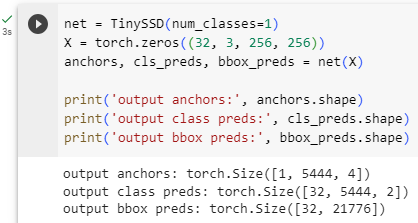
As shown earlier in this section, the first block outputs 32×32 feature maps. Recall that the second to fourth downsampling blocks halve the height and width and the fifth block uses global pooling. Since 4 anchor boxes are generated for each unit along spatial dimensions of feature maps, at all the five scales a total of (322+162+82+42+1)×4=5444 anchor boxes are generated for each image.
이 섹션의 앞부분에 표시된 것처럼 첫 번째 블록은 32×32 기능 맵을 출력합니다. 두 번째에서 네 번째 다운샘플링 블록은 높이와 너비를 절반으로 줄이고 다섯 번째 블록은 전역 풀링을 사용한다는 점을 기억하세요. 특징 맵의 공간 차원을 따라 각 단위에 대해 4개의 앵커 상자가 생성되므로 모든 5개 축척에서 각 이미지에 대해 총 (322+162+82+42+1)×4=5444개의 앵커 상자가 생성됩니다.
net = TinySSD(num_classes=1)
X = torch.zeros((32, 3, 256, 256))
anchors, cls_preds, bbox_preds = net(X)

print('output anchors:', anchors.shape)
print('output class preds:', cls_preds.shape)
print('output bbox preds:', bbox_preds.shape)- net = TinySSD(num_classes=1): TinySSD 클래스를 사용하여 객체 검출을 위한 작은 SSD 모델 net을 생성합니다. num_classes=1은 검출하려는 클래스의 개수를 1로 설정한다는 의미입니다.
- X = torch.zeros((32, 3, 256, 256)): 크기가 32x3x256x256인 입력 데이터 X를 생성합니다. 이 입력 데이터는 배치 크기가 32이고 채널 수가 3인 이미지로 구성되며, 이미지의 가로 및 세로 크기는 각각 256입니다.
- anchors, cls_preds, bbox_preds = net(X): 생성한 모델 net에 입력 데이터 X를 통과시켜 앵커, 클래스 예측값, 바운딩 박스 예측값을 얻습니다. anchors, cls_preds, bbox_preds 변수에 각각의 결과가 할당됩니다.
- print('output anchors:', anchors.shape): anchors의 크기를 출력합니다. 이 부분은 네트워크의 순전파 결과로 생성된 앵커의 크기를 확인하는 역할을 합니다.
- print('output class preds:', cls_preds.shape): cls_preds의 크기를 출력합니다. 이 부분은 네트워크의 순전파 결과로 생성된 클래스 예측값의 크기를 확인하는 역할을 합니다.
- print('output bbox preds:', bbox_preds.shape): bbox_preds의 크기를 출력합니다. 이 부분은 네트워크의 순전파 결과로 생성된 바운딩 박스 예측값의 크기를 확인하는 역할을 합니다.
이 코드는 작은 SSD 모델에 입력 데이터를 통과시켜 앵커, 클래스 예측값, 바운딩 박스 예측값을 생성하고, 각 결과의 크기를 확인하는 역할을 수행합니다.
14.7.2. Training
Now we will explain how to train the single shot multibox detection model for object detection.
이제 객체 감지를 위해 단일 샷 멀티박스 감지 모델을 훈련하는 방법을 설명합니다.
14.7.2.1. Reading the Dataset and Initializing the Model
To begin with, let’s read the banana detection dataset described in Section 14.6.
먼저 섹션 14.6에 설명된 바나나 감지 데이터 세트를 읽어 보겠습니다.
batch_size = 32
train_iter, _ = d2l.load_data_bananas(batch_size)- batch_size = 32: 배치 크기를 32로 설정합니다. 배치 크기는 한 번의 학습 단계에서 처리되는 데이터의 개수를 나타냅니다. 여기서는 32개의 데이터가 하나의 배치로 묶여 처리될 것입니다.
- train_iter, _ = d2l.load_data_bananas(batch_size): d2l.load_data_bananas(batch_size) 함수를 호출하여 바나나 객체 검출 데이터셋을 로드합니다. 이 함수는 학습 데이터를 미니배치로 나누어 제공하는 데이터 로더를 생성합니다. 여기서 반환되는 train_iter는 학습 데이터셋의 미니배치를 순회하는 반복자(iterator)입니다. 코드에서 _는 두 번째 반환값을 무시하는 변수입니다. 이렇게 생성된 데이터 로더를 사용하여 모델을 학습하게 될 것입니다.
이 코드는 배치 크기를 설정하고 바나나 객체 검출 데이터셋을 미니배치로 나누어 학습용 데이터 로더를 생성하는 역할을 합니다.

There is only one class in the banana detection dataset. After defining the model, we need to initialize its parameters and define the optimization algorithm.
바나나 감지 데이터 세트에는 하나의 클래스만 있습니다. 모델을 정의한 후 매개변수를 초기화하고 최적화 알고리즘을 정의해야 합니다.
device, net = d2l.try_gpu(), TinySSD(num_classes=1)
trainer = torch.optim.SGD(net.parameters(), lr=0.2, weight_decay=5e-4)- device, net = d2l.try_gpu(), TinySSD(num_classes=1): d2l.try_gpu() 함수를 사용하여 GPU 디바이스를 시도하고, 그 결과를 device 변수에 저장합니다. 그 다음, TinySSD 클래스를 사용하여 객체 검출을 위한 작은 SSD 모델 net을 생성합니다. num_classes=1은 검출하려는 클래스의 개수를 1로 설정한다는 의미입니다.
- trainer = torch.optim.SGD(net.parameters(), lr=0.2, weight_decay=5e-4): torch.optim.SGD를 사용하여 확률적 경사 하강법(Stochastic Gradient Descent) 옵티마이저 trainer를 생성합니다. net.parameters()는 모델의 학습 가능한 매개변수들을 가져옵니다. lr=0.2는 학습률(learning rate)을 0.2로 설정한다는 의미이며, weight_decay=5e-4는 L2 정규화를 위한 가중치 감쇠(weight decay)를 설정합니다. 이 옵티마이저는 모델을 학습할 때 매개변수 업데이트를 수행하는데 사용됩니다.
이 코드는 GPU 디바이스를 시도하고 작은 SSD 모델을 생성한 후, 확률적 경사 하강법 옵티마이저를 설정하는 역할을 합니다. 이러한 설정을 통해 모델을 GPU로 이동하고, 옵티마이저를 사용하여 모델의 학습 과정을 설정합니다.
14.7.2.2. Defining Loss and Evaluation Functions
Object detection has two types of losses. The first loss concerns classes of anchor boxes: its computation can simply reuse the cross-entropy loss function that we used for image classification. The second loss concerns offsets of positive (non-background) anchor boxes: this is a regression problem. For this regression problem, however, here we do not use the squared loss described in Section 3.1.3. Instead, we use the ℓ1 norm loss, the absolute value of the difference between the prediction and the ground-truth. The mask variable bbox_masks filters out negative anchor boxes and illegal (padded) anchor boxes in the loss calculation. In the end, we sum up the anchor box class loss and the anchor box offset loss to obtain the loss function for the model.
객체 감지에는 두 가지 유형의 손실이 있습니다. 첫 번째 손실은 앵커 박스의 클래스와 관련이 있습니다. 해당 계산은 이미지 분류에 사용한 교차 엔트로피 손실 함수를 단순히 재사용할 수 있습니다. 두 번째 손실은 포지티브(배경이 아닌) 앵커 상자의 오프셋과 관련됩니다. 이것은 회귀 문제입니다. 그러나이 회귀 문제의 경우 여기에서는 섹션 3.1.3에서 설명한 제곱 손실을 사용하지 않습니다. 대신, 우리는 예측과 ground-truth 사이의 차이의 절대값인 ℓ1 놈 손실을 사용합니다. 마스크 변수 bbox_masks는 손실 계산에서 음의 앵커 상자와 불법(패딩된) 앵커 상자를 필터링합니다. 마지막으로 앵커 박스 클래스 손실과 앵커 박스 오프셋 손실을 합산하여 모델에 대한 손실 함수를 얻습니다.
cls_loss = nn.CrossEntropyLoss(reduction='none')
bbox_loss = nn.L1Loss(reduction='none')

def calc_loss(cls_preds, cls_labels, bbox_preds, bbox_labels, bbox_masks):
    batch_size, num_classes = cls_preds.shape[0], cls_preds.shape[2]
    cls = cls_loss(cls_preds.reshape(-1, num_classes),
                   cls_labels.reshape(-1)).reshape(batch_size, -1).mean(dim=1)
    bbox = bbox_loss(bbox_preds * bbox_masks,
                     bbox_labels * bbox_masks).mean(dim=1)
return cls + bbox- cls_loss = nn.CrossEntropyLoss(reduction='none'): nn.CrossEntropyLoss 함수를 사용하여 클래스 예측값과 클래스 실제값 사이의 손실(loss)를 계산하는데 사용될 cls_loss를 정의합니다. reduction='none'은 손실을 각 샘플에 대해 개별적으로 계산하겠다는 의미입니다.
- bbox_loss = nn.L1Loss(reduction='none'): nn.L1Loss 함수를 사용하여 바운딩 박스 예측값과 실제 바운딩 박스 사이의 L1 손실(loss)를 계산하는데 사용될 bbox_loss를 정의합니다. reduction='none'은 손실을 각 샘플에 대해 개별적으로 계산하겠다는 의미입니다.
- def calc_loss(cls_preds, cls_labels, bbox_preds, bbox_labels, bbox_masks):: 손실을 계산하는 함수를 정의합니다. 이 함수는 클래스 예측값, 클래스 실제값, 바운딩 박스 예측값, 바운딩 박스 실제값, 바운딩 박스 마스크를 입력으로 받습니다.
- batch_size, num_classes = cls_preds.shape[0], cls_preds.shape[2]: 배치 크기와 클래스 개수를 가져옵니다.
- cls_loss(cls_preds.reshape(-1, num_classes), cls_labels.reshape(-1)): 클래스 예측값과 실제값을 모양을 변형하여 크로스 엔트로피 손실을 계산합니다. reshape(-1, num_classes)는 데이터를 배치 크기와 클래스 개수에 맞게 재구성하여 계산합니다.
- .reshape(batch_size, -1).mean(dim=1): 계산된 클래스 손실을 다시 배치 크기에 맞게 재구성하고, 각 배치의 평균을 계산합니다.
- bbox_loss(bbox_preds * bbox_masks, bbox_labels * bbox_masks).mean(dim=1): 바운딩 박스 예측값과 실제값에 바운딩 박스 마스크를 적용하여 L1 손실을 계산하고, 각 배치의 평균을 계산합니다.
- return cls + bbox: 클래스 손실과 바운딩 박스 손실을 더하여 최종 손실을 반환합니다.
이 함수는 클래스 예측과 바운딩 박스 예측 간의 손실을 계산하는데 사용되며, 클래스 손실과 바운딩 박스 손실을 더하여 최종적인 학습 손실을 계산하는 역할을 합니다.
We can use accuracy to evaluate the classification results. Due to the used ℓ1 norm loss for the offsets, we use the mean absolute error to evaluate the predicted bounding boxes. These prediction results are obtained from the generated anchor boxes and the predicted offsets for them.
정확도를 사용하여 분류 결과를 평가할 수 있습니다. 오프셋에 사용된 ℓ1 노름 손실로 인해 예측된 경계 상자를 평가하기 위해 평균 절대 오차를 사용합니다. 이러한 예측 결과는 생성된 앵커 박스와 그에 대한 예측된 오프셋에서 얻습니다.
def cls_eval(cls_preds, cls_labels):
    # Because the class prediction results are on the final dimension,
    # `argmax` needs to specify this dimension
    return float((cls_preds.argmax(dim=-1).type(
        cls_labels.dtype) == cls_labels).sum())

def bbox_eval(bbox_preds, bbox_labels, bbox_masks):
return float((torch.abs((bbox_labels - bbox_preds) * bbox_masks)).sum())- def cls_eval(cls_preds, cls_labels):: 클래스 예측값과 실제 클래스 레이블 사이의 일치 여부를 평가하는 함수를 정의합니다. 이 함수는 클래스 예측값, 실제 클래스 레이블을 입력으로 받습니다.
- cls_preds.argmax(dim=-1): 클래스 예측값에서 가장 높은 값의 인덱스를 찾습니다. 여기서 dim=-1은 마지막 차원을 기준으로 최대값을 찾는다는 의미입니다.
- .type(cls_labels.dtype) == cls_labels: 클래스 예측값의 최대 인덱스와 실제 클래스 레이블이 같은지를 비교합니다. 이 결과는 불리언 값으로 반환됩니다.
- .sum(): 불리언 값을 모두 합산하여 일치하는 클래스 개수를 구합니다.
- return float(...): 일치하는 클래스 개수를 부동소수점 형태로 반환합니다.
- def bbox_eval(bbox_preds, bbox_labels, bbox_masks):: 바운딩 박스 예측값과 실제 바운딩 박스 레이블 사이의 차이를 평가하는 함수를 정의합니다. 이 함수는 바운딩 박스 예측값, 실제 바운딩 박스 레이블, 바운딩 박스 마스크를 입력으로 받습니다.
- torch.abs((bbox_labels - bbox_preds) * bbox_masks): 실제 바운딩 박스 레이블과 예측 바운딩 박스 값 사이의 차이를 계산하고, 이를 바운딩 박스 마스크와 곱하여 차이를 마스크된 영역에만 적용합니다. 이렇게 계산된 결과는 절댓값을 취합니다.
- .sum(): 절댓값 차이를 모두 합산하여 바운딩 박스 예측과 실제 값 사이의 차이를 구합니다.
- return float(...): 바운딩 박스 값의 차이를 부동소수점 형태로 반환합니다.
이러한 함수들은 클래스 예측과 바운딩 박스 예측의 정확도와 일치도를 평가하는 데 사용됩니다. cls_eval 함수는 클래스 예측 정확도를 평가하고, bbox_eval 함수는 바운딩 박스 예측과 실제 값 사이의 차이를 평가합니다.
14.7.2.3. Training the Model
When training the model, we need to generate multiscale anchor boxes (anchors) and predict their classes (cls_preds) and offsets (bbox_preds) in the forward propagation. Then we label the classes (cls_labels) and offsets (bbox_labels) of such generated anchor boxes based on the label information Y. Finally, we calculate the loss function using the predicted and labeled values of the classes and offsets. For concise implementations, evaluation of the test dataset is omitted here.
모델을 교육할 때 다중 스케일 앵커 상자(앵커)를 생성하고 순방향 전파에서 해당 클래스(cls_preds) 및 오프셋(bbox_preds)을 예측해야 합니다. 그런 다음 레이블 정보 Y를 기반으로 이렇게 생성된 앵커 박스의 클래스(cls_labels)와 오프셋(bbox_labels)에 레이블을 지정합니다. 마지막으로 클래스와 오프셋의 예측 및 레이블 값을 사용하여 손실 함수를 계산합니다. 간결한 구현을 위해 테스트 데이터 세트의 평가는 여기에서 생략됩니다.
num_epochs, timer = 20, d2l.Timer()
animator = d2l.Animator(xlabel='epoch', xlim=[1, num_epochs],
                        legend=['class error', 'bbox mae'])
net = net.to(device)
for epoch in range(num_epochs):
    # Sum of training accuracy, no. of examples in sum of training accuracy,
    # Sum of absolute error, no. of examples in sum of absolute error
    metric = d2l.Accumulator(4)
    net.train()
    for features, target in train_iter:
        timer.start()
        trainer.zero_grad()
        X, Y = features.to(device), target.to(device)
        # Generate multiscale anchor boxes and predict their classes and
        # offsets
        anchors, cls_preds, bbox_preds = net(X)
        # Label the classes and offsets of these anchor boxes
        bbox_labels, bbox_masks, cls_labels = d2l.multibox_target(anchors, Y)
        # Calculate the loss function using the predicted and labeled values
        # of the classes and offsets
        l = calc_loss(cls_preds, cls_labels, bbox_preds, bbox_labels,
                      bbox_masks)
        l.mean().backward()
        trainer.step()
        metric.add(cls_eval(cls_preds, cls_labels), cls_labels.numel(),
                   bbox_eval(bbox_preds, bbox_labels, bbox_masks),
                   bbox_labels.numel())
    cls_err, bbox_mae = 1 - metric[0] / metric[1], metric[2] / metric[3]
    animator.add(epoch + 1, (cls_err, bbox_mae))
print(f'class err {cls_err:.2e}, bbox mae {bbox_mae:.2e}')
print(f'{len(train_iter.dataset) / timer.stop():.1f} examples/sec on '
f'{str(device)}')- num_epochs, timer = 20, d2l.Timer(): 학습 에포크 수를 20으로 설정하고, 시간 측정을 위한 d2l.Timer() 객체를 생성합니다.
- animator = d2l.Animator(xlabel='epoch', xlim=[1, num_epochs], legend=['class error', 'bbox mae']): 그래프를 그리기 위한 d2l.Animator() 객체를 생성합니다. 이 그래프는 에포크별 클래스 오류와 바운딩 박스 평균 절대 오차(MAE)를 나타낼 것입니다.
- net = net.to(device): 모델 net을 GPU 디바이스로 이동시킵니다.
- for epoch in range(num_epochs):: 에포크 수만큼 반복합니다.
- metric = d2l.Accumulator(4): 훈련 중에 모니터링할 메트릭 값을 저장할 d2l.Accumulator() 객체를 생성합니다. 이 메트릭은 훈련 정확도, 훈련 정확도의 샘플 개수, 절댓값 오차, 절댓값 오차의 샘플 개수를 나타냅니다.
- net.train(): 모델을 훈련 모드로 설정합니다.
- for features, target in train_iter:: 훈련 데이터 로더에서 미니배치를 가져옵니다.
- timer.start(): 시간 측정을 시작합니다.
- trainer.zero_grad(): 옵티마이저의 그라디언트를 초기화합니다.
- X, Y = features.to(device), target.to(device): 입력 데이터와 레이블을 GPU 디바이스로 이동시킵니다.
- anchors, cls_preds, bbox_preds = net(X): 입력 데이터를 모델에 통과시켜 앵커, 클래스 예측값, 바운딩 박스 예측값을 얻습니다.
- bbox_labels, bbox_masks, cls_labels = d2l.multibox_target(anchors, Y): 앵커와 레이블을 이용하여 바운딩 박스 레이블, 바운딩 박스 마스크, 클래스 레이블을 생성합니다.
- l = calc_loss(...): 계산된 레이블과 예측값을 사용하여 손실 함수를 계산합니다.
- l.mean().backward(): 손실의 평균을 구하고, 역전파를 수행합니다.
- trainer.step(): 옵티마이저를 사용하여 모델의 매개변수를 업데이트합니다.
- metric.add(...): 훈련 중에 계산된 메트릭 값을 누적합니다. 클래스 정확도와 바운딩 박스 MAE를 계산하여 누적합니다.
- cls_err, bbox_mae = ...: 에포크별 클래스 오류와 바운딩 박스 평균 절대 오차를 계산합니다.
- animator.add(...): 그래프를 그리기 위해 그래프 데이터를 추가합니다. 에포크와 클래스 오류, 바운딩 박스 MAE를 그래프에 추가합니다.
- print(f'class err {cls_err:.2e}, bbox mae {bbox_mae:.2e}'): 학습 종료 후, 최종 클래스 오류와 바운딩 박스 MAE를 출력합니다.
- print(f'{len(train_iter.dataset) / timer.stop():.1f} examples/sec on ' f'{str(device)}'): 학습 속도를 출력합니다. 데이터셋에 대한 처리 속도와 사용한 디바이스(GPU) 정보도 함께 출력합니다.
이 코드는 작은 SSD 모델을 학습하는 주요 학습 루프를 나타내며, 각 에포크마다 클래스 오류와 바운딩 박스 MAE를 계산하여 모니터링합니다.


14.7.3. Prediction
During prediction, the goal is to detect all the objects of interest on the image. Below we read and resize a test image, converting it to a four-dimensional tensor that is required by convolutional layers.
예측하는 동안 목표는 이미지에서 관심 대상을 모두 감지하는 것입니다. 아래에서는 테스트 이미지를 읽고 크기를 조정하여 컨볼루션 레이어에 필요한 4차원 텐서로 변환합니다.
X = torchvision.io.read_image('../img/banana.jpg').unsqueeze(0).float()
img = X.squeeze(0).permute(1, 2, 0).long()
Using the multibox_detection function below, the predicted bounding boxes are obtained from the anchor boxes and their predicted offsets. Then non-maximum suppression is used to remove similar predicted bounding boxes.
아래의 multibox_detection 함수를 사용하여 앵커 박스와 예측된 오프셋에서 예측된 경계 상자를 얻습니다. 그런 다음 유사한 예측 경계 상자를 제거하기 위해 최대가 아닌 억제가 사용됩니다.
def predict(X):
    net.eval()
    anchors, cls_preds, bbox_preds = net(X.to(device))
    cls_probs = F.softmax(cls_preds, dim=2).permute(0, 2, 1)
    output = d2l.multibox_detection(cls_probs, bbox_preds, anchors)
    idx = [i for i, row in enumerate(output[0]) if row[0] != -1]
    return output[0, idx]

output = predict(X)- def predict(X):: 입력 이미지 X에 대한 객체 검출 예측을 수행하는 함수를 정의합니다.
- net.eval(): 모델을 평가 모드로 설정합니다. 평가 모드에서는 드롭아웃이나 배치 정규화와 같은 레이어의 동작이 변경되어 평가에 적합하게 동작합니다.
- anchors, cls_preds, bbox_preds = net(X.to(device)): 입력 이미지를 모델에 통과시켜 앵커, 클래스 예측값, 바운딩 박스 예측값을 얻습니다. X를 GPU 디바이스로 이동시켜 계산합니다.
- cls_probs = F.softmax(cls_preds, dim=2).permute(0, 2, 1): 클래스 예측값에 소프트맥스 함수를 적용하여 클래스 확률을 계산합니다. dim=2는 클래스 차원을 기준으로 소프트맥스를 계산한다는 의미이며, .permute(0, 2, 1)은 클래스 차원을 뒤로 옮깁니다.
- output = d2l.multibox_detection(cls_probs, bbox_preds, anchors): 클래스 확률과 바운딩 박스 예측값, 앵커 정보를 이용하여 객체 검출을 수행합니다. 이 함수는 객체 검출 결과를 반환합니다.
- idx = [i for i, row in enumerate(output[0]) if row[0] != -1]: 검출 결과 중에서 신뢰도가 -1이 아닌 객체 인덱스를 찾습니다.
- return output[0, idx]: 신뢰도가 -1이 아닌 객체에 대한 검출 결과를 반환합니다.
- output = predict(X): 입력 이미지 X에 대한 객체 검출을 수행하여 결과를 output에 저장합니다.
이 코드는 학습된 모델을 사용하여 입력 이미지에 대한 객체 검출을 수행하고, 결과를 반환하는 함수를 정의하며, 실제로 객체 검출을 수행하여 결과를 output에 저장하는 과정을 나타냅니다.
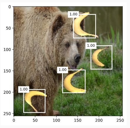
Finally, we display all the predicted bounding boxes with confidence 0.9 or above as output.
마지막으로 신뢰도가 0.9 이상인 모든 예측 경계 상자를 출력으로 표시합니다.
def display(img, output, threshold):
    d2l.set_figsize((5, 5))
    fig = d2l.plt.imshow(img)
    for row in output:
        score = float(row[1])
        if score < threshold:
            continue
        h, w = img.shape[:2]
        bbox = [row[2:6] * torch.tensor((w, h, w, h), device=row.device)]
        d2l.show_bboxes(fig.axes, bbox, '%.2f' % score, 'w')

display(img, output.cpu(), threshold=0.9)- def display(img, output, threshold):: 입력 이미지 img와 객체 검출 결과 output, 그리고 신뢰도 임계값 threshold를 받아 객체 검출 결과를 시각화하는 함수를 정의합니다.
- d2l.set_figsize((5, 5)): 그림 크기를 설정합니다.
- fig = d2l.plt.imshow(img): 입력 이미지를 Matplotlib의 이미지로 표시하고, 해당 이미지 객체를 fig에 저장합니다.
- for row in output:: 객체 검출 결과 output의 각 행에 대해서 반복합니다.
- score = float(row[1]): 객체 검출 결과에서 신뢰도를 가져옵니다. row[1]은 신뢰도 값을 나타냅니다.
- if score < threshold:: 만약 신뢰도가 임계값보다 작으면 넘어갑니다.
- h, w = img.shape[:2]: 입력 이미지의 높이와 너비를 가져옵니다.
- bbox = [row[2:6] * torch.tensor((w, h, w, h), device=row.device)]: 객체 검출 결과에서 바운딩 박스 정보를 가져온 후, 바운딩 박스 좌표를 이미지 크기에 맞게 스케일 조정합니다.
- d2l.show_bboxes(fig.axes, bbox, '%.2f' % score, 'w'): 스케일 조정된 바운딩 박스와 신뢰도 값을 사용하여 Matplotlib의 축에 바운딩 박스와 레이블을 표시합니다.
- display(img, output.cpu(), threshold=0.9): 입력 이미지 img와 객체 검출 결과 output를 시각화합니다. 여기서 output의 텐서를 CPU로 이동시켜야 Matplotlib과 호환됩니다. 신뢰도 임계값은 0.9로 설정되어 0.9보다 높은 신뢰도를 가진 객체만 표시됩니다.
이 코드는 객체 검출 결과를 시각화하여 신뢰도 임계값을 넘는 객체들을 표시하는 함수를 정의하고, 실제 이미지와 객체 검출 결과를 사용하여 시각화하는 과정을 나타냅니다.
14.7.4. Summary
- Single shot multibox detection is a multiscale object detection model. Via its base network and several multiscale feature map blocks, single-shot multibox detection generates a varying number of anchor boxes with different sizes, and detects varying-size objects by predicting classes and offsets of these anchor boxes (thus the bounding boxes).
- 단일 샷 멀티박스 감지는 다중 스케일 객체 감지 모델입니다. 기본 네트워크와 여러 멀티스케일 기능 맵 블록을 통해 단일 샷 멀티박스 감지는 다양한 크기의 다양한 앵커 박스를 생성하고 이러한 앵커 박스(따라서 경계 박스)의 클래스와 오프셋을 예측하여 다양한 크기의 객체를 감지합니다.
- When training the single-shot multibox detection model, the loss function is calculated based on the predicted and labeled values of the anchor box classes and offsets.
- 단일 샷 멀티박스 감지 모델을 훈련할 때 손실 함수는 앵커 박스 클래스 및 오프셋의 예측 및 레이블 값을 기반으로 계산됩니다.
14.7.5. Exercises
- Can you improve the single-shot multibox detection by improving the loss function? For example, replace ℓ1 norm loss with smooth ℓ1 norm loss for the predicted offsets. This loss function uses a square function around zero for smoothness, which is controlled by the hyperparameter σ:

When σ is very large, this loss is similar to the ℓ1 norm loss. When its value is smaller, the loss function is smoother.
def smooth_l1(data, scalar):
    out = []
    for i in data:
        if abs(i) < 1 / (scalar ** 2):
            out.append(((scalar * i) ** 2) / 2)
        else:
            out.append(abs(i) - 0.5 / (scalar ** 2))
    return torch.tensor(out)

sigmas = [10, 1, 0.5]
lines = ['-', '--', '-.']
x = torch.arange(-2, 2, 0.1)
d2l.set_figsize()

for l, s in zip(lines, sigmas):
    y = smooth_l1(x, scalar=s)
    d2l.plt.plot(x, y, l, label='sigma=%.1f' % s)
d2l.plt.legend();- def smooth_l1(data, scalar):: 입력 데이터 data와 스칼라 값 scalar를 받아서 smooth L1 손실 함수 값을 계산하는 함수를 정의합니다.
- out = []: 결과 값을 저장할 빈 리스트를 생성합니다.
- for i in data:: 입력 데이터의 각 원소에 대해서 반복합니다.
- if abs(i) < 1 / (scalar ** 2):: 만약 입력 데이터의 절댓값이 1 / (scalar ** 2)보다 작으면,
- out.append(((scalar * i) ** 2) / 2): 출력 리스트에 (scalar * i)^2 / 2 값을 추가합니다.
- else:: 그렇지 않으면,
- out.append(abs(i) - 0.5 / (scalar ** 2)): 출력 리스트에 abs(i) - 0.5 / (scalar ** 2) 값을 추가합니다.
- if abs(i) < 1 / (scalar ** 2):: 만약 입력 데이터의 절댓값이 1 / (scalar ** 2)보다 작으면,
- return torch.tensor(out): 계산된 결과를 텐서 형태로 반환합니다.
- sigmas = [10, 1, 0.5]: 다양한 시그마 값 리스트를 정의합니다.
- lines = ['-', '--', '-.']: 그래프에서 사용할 라인 스타일을 정의합니다.
- x = torch.arange(-2, 2, 0.1): -2부터 2까지 0.1 간격으로 숫자들을 생성하여 x를 정의합니다.
- d2l.set_figsize(): 그래프 크기를 설정합니다.
- for l, s in zip(lines, sigmas):: 라인 스타일과 시그마 값을 하나씩 가져오면서 반복합니다.
- y = smooth_l1(x, scalar=s): smooth_l1 함수를 사용하여 x 값에 대한 smooth L1 손실 함수 값을 계산하여 y에 저장합니다.
- d2l.plt.plot(x, y, l, label='sigma=%.1f' % s): 계산된 x와 y 값을 사용하여 그래프를 그리고, 라벨에 시그마 값을 표시합니다.
- d2l.plt.legend(): 그래프에 범례를 표시합니다.
이 코드는 다양한 시그마 값을 사용하여 smooth L1 손실 함수를 그래프로 표현하는 작업을 수행합니다.


def focal_loss(gamma, x):
    return -(1 - x) ** gamma * torch.log(x)

x = torch.arange(0.01, 1, 0.01)
for l, gamma in zip(lines, [0, 1, 5]):
    y = d2l.plt.plot(x, focal_loss(gamma, x), l, label='gamma=%.1f' % gamma)
d2l.plt.legend();- def focal_loss(gamma, x):: 파라미터 gamma와 입력 x를 받아 focal loss 값을 계산하는 함수를 정의합니다.
- return -(1 - x) ** gamma * torch.log(x): focal loss를 계산하여 반환합니다. focal loss는 -(1 - x)^gamma * log(x) 형태로 정의됩니다.
- x = torch.arange(0.01, 1, 0.01): 0.01부터 1까지 0.01 간격으로 숫자들을 생성하여 x를 정의합니다.
- for l, gamma in zip(lines, [0, 1, 5]):: 라인 스타일과 감마 값을 하나씩 가져오면서 반복합니다.
- y = d2l.plt.plot(x, focal_loss(gamma, x), l, label='gamma=%.1f' % gamma): x 값에 대해 해당 감마 값을 사용하여 focal loss를 계산하고, 그래프를 그립니다. 라벨에 감마 값을 표시합니다.
- d2l.plt.legend(): 그래프에 범례를 표시합니다.
이 코드는 다양한 감마 값과 입력에 대한 focal loss 함수를 그래프로 표현하는 작업을 수행합니다.

- Due to space limitations, we have omitted some implementation details of the single shot multibox detection model in this section. Can you further improve the model in the following aspects:
- When an object is much smaller compared with the image, the model could resize the input image bigger.
- There are typically a vast number of negative anchor boxes. To make the class distribution more balanced, we could downsample negative anchor boxes.
- In the loss function, assign different weight hyperparameters to the class loss and the offset loss.
- Use other methods to evaluate the object detection model, such as those in the single shot multibox detection paper (Liu et al., 2016).
'Dive into Deep Learning > D2L Computer Vision' 카테고리의 다른 글
| D2L - 14.12. Neural Style Transfer (1) | 2023.08.21 |
|---|---|
| D2L - 14.11. Fully Convolutional Networks (0) | 2023.08.21 |
| D2L - 14.10. Transposed Convolution (1) | 2023.08.21 |
| D2L - 14.9. Semantic Segmentation and the Dataset (0) | 2023.08.20 |
| D2L - 14.8. Region-based CNNs (R-CNNs) (0) | 2023.08.20 |
| D2L - 14.6. The Object Detection Dataset (0) | 2023.08.19 |
| D2L - 14.5. Multiscale Object Detection (0) | 2023.08.19 |
| D2L - 14.4. Anchor Boxes (0) | 2023.08.19 |
| D2L - 14.3. Object Detection and Bounding Boxes (0) | 2023.08.19 |
| D2L - 14.2. Fine-Tuning (0) | 2023.08.19 |