

https://d2l.ai/chapter_computer-vision/fine-tuning.html
14.2. Fine-Tuning — Dive into Deep Learning 1.0.0 documentation
d2l.ai
14.2. Fine-Tuning
In earlier chapters, we discussed how to train models on the Fashion-MNIST training dataset with only 60000 images. We also described ImageNet, the most widely used large-scale image dataset in academia, which has more than 10 million images and 1000 objects. However, the size of the dataset that we usually encounter is between those of the two datasets.
이전 장에서 60000개의 이미지만으로 Fashion-MNIST 교육 데이터 세트에서 모델을 교육하는 방법에 대해 논의했습니다. 또한 학계에서 가장 널리 사용되는 대규모 이미지 데이터 세트인 ImageNet에 대해서도 설명했습니다. 이 데이터 세트에는 천만 개 이상의 이미지와 1000개 개체가 있습니다. 그러나 우리가 일반적으로 접하는 데이터 세트의 크기는 두 데이터 세트의 중간 크기입니다.
Suppose that we want to recognize different types of chairs from images, and then recommend purchase links to users. One possible method is to first identify 100 common chairs, take 1000 images of different angles for each chair, and then train a classification model on the collected image dataset. Although this chair dataset may be larger than the Fashion-MNIST dataset, the number of examples is still less than one-tenth of that in ImageNet. This may lead to overfitting of complicated models that are suitable for ImageNet on this chair dataset. Besides, due to the limited amount of training examples, the accuracy of the trained model may not meet practical requirements.
이미지에서 다양한 유형의 의자를 인식하고 사용자에게 구매 링크를 추천하고 싶다고 가정합니다. 한 가지 가능한 방법은 먼저 100개의 일반적인 의자를 식별하고 각 의자에 대해 서로 다른 각도의 이미지 1000개를 가져온 다음 수집된 이미지 데이터 세트에서 분류 모델을 훈련하는 것입니다. 이 의자 데이터셋은 Fashion-MNIST 데이터셋보다 클 수 있지만 예제의 수는 여전히 ImageNet의 1/10 미만입니다. 이로 인해 이 의자 데이터 세트에서 ImageNet에 적합한 복잡한 모델이 과대적합될 수 있습니다. 게다가 제한된 양의 학습 예제로 인해 학습된 모델의 정확도가 실제 요구 사항을 충족하지 못할 수 있습니다.
In order to address the above problems, an obvious solution is to collect more data. However, collecting and labeling data can take a lot of time and money. For example, in order to collect the ImageNet dataset, researchers have spent millions of dollars from research funding. Although the current data collection cost has been significantly reduced, this cost still cannot be ignored.
위의 문제를 해결하기 위한 확실한 해결책은 더 많은 데이터를 수집하는 것입니다. 그러나 데이터를 수집하고 레이블을 지정하는 데는 많은 시간과 비용이 소요될 수 있습니다. 예를 들어 ImageNet 데이터 세트를 수집하기 위해 연구자들은 연구 자금에서 수백만 달러를 지출했습니다. 현재 데이터 수집 비용이 크게 줄었지만 이 비용은 여전히 무시할 수 없습니다.
Another solution is to apply transfer learning to transfer the knowledge learned from the source dataset to the target dataset. For example, although most of the images in the ImageNet dataset have nothing to do with chairs, the model trained on this dataset may extract more general image features, which can help identify edges, textures, shapes, and object composition. These similar features may also be effective for recognizing chairs.
또 다른 해결책은 전이 학습(transfer learning)을 적용하여 원본 데이터 세트에서 학습한 지식을 대상 데이터 세트로 이전하는 것입니다. 예를 들어 ImageNet 데이터세트의 대부분의 이미지는 의자와 관련이 없지만 이 데이터세트에서 훈련된 모델은 가장자리, 질감, 모양 및 개체 구성을 식별하는 데 도움이 될 수 있는 보다 일반적인 이미지 기능을 추출할 수 있습니다. 이러한 유사한 기능은 의자를 인식하는 데에도 효과적일 수 있습니다.
Transfer Learning (전이 학습) 이란?
'transfer learning(전이 학습)'은 하나의 작업에서 학습한 모델의 지식을 다른 관련 작업으로 전달하여 학습하는 기술을 말합니다. 기존에 학습된 모델의 일부 또는 전체 네트워크 구조와 가중치를 새로운 작업에 재사용하는 것을 의미합니다. 이를 통해 새로운 작업에 대한 학습 데이터가 부족한 경우에도 모델의 성능을 향상시킬 수 있습니다.
전이 학습은 다음과 같은 장점을 가지고 있습니다:
- 데이터 부족 문제 해결: 새로운 작업에 충분한 양의 학습 데이터가 없을 때, 기존 작업에서 학습한 모델을 전이하여 성능을 향상시킬 수 있습니다.
- 학습 시간 단축: 기존에 학습된 모델의 가중치를 초기화로 사용하면 초기 모델의 성능은 높아지며, 새로운 작업에 대한 학습 시간을 단축할 수 있습니다.
- 일반화 능력 향상: 기존 작업에서 학습한 모델은 이미 다양한 특징을 학습했으므로 이를 활용하여 새로운 작업에서의 성능을 향상시킬 수 있습니다.
전이 학습은 이미지 분류, 객체 검출, 자연어 처리 등 다양한 분야에서 활용되며, 사전 학습된 모델을 가져와서 적절한 수정 및 조정을 통해 새로운 작업에 맞게 재사용하는 것이 일반적인 접근 방식입니다.
14.2.1. Steps
In this section, we will introduce a common technique in transfer learning: fine-tuning. As shown in Fig. 14.2.1, fine-tuning consists of the following four steps:
이 섹션에서는 전이 학습의 일반적인 기술인 미세 조정을 소개합니다. 그림 14.2.1과 같이 미세 조정은 다음 네 단계로 구성됩니다.
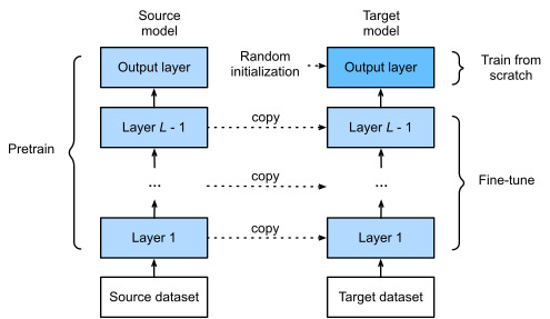
When target datasets are much smaller than source datasets, fine-tuning helps to improve models’ generalization ability.
대상 데이터 세트가 소스 데이터 세트보다 훨씬 작을 때 미세 조정하면 모델의 일반화 능력을 향상시키는 데 도움이 됩니다.
14.2.2. Hot Dog Recognition
Let’s demonstrate fine-tuning via a concrete case: hot dog recognition. We will fine-tune a ResNet model on a small dataset, which was pretrained on the ImageNet dataset. This small dataset consists of thousands of images with and without hot dogs. We will use the fine-tuned model to recognize hot dogs from images.
핫도그 인식이라는 구체적인 사례를 통해 미세 조정을 시연해 보겠습니다. ImageNet 데이터 세트에서 사전 훈련된 작은 데이터 세트에서 ResNet 모델을 미세 조정합니다. 이 작은 데이터 세트는 핫도그가 있거나 없는 수천 개의 이미지로 구성됩니다. 미세 조정된 모델을 사용하여 이미지에서 핫도그를 인식합니다.
%matplotlib inline
import os
import torch
import torchvision
from torch import nn
from d2l import torch as d2l
이 코드는 딥러닝 모델을 구축하고 학습하기 위해 필요한 라이브러리와 설정을 불러오는 부분입니다. 각 줄의 역할을 살펴보겠습니다:
- %matplotlib inline: 이 코드는 주피터 노트북 상에서 그래프를 인라인으로 표시하도록 설정하는 매직 명령어입니다. 따라서 그래프를 그릴 때 별도의 창이 아니라 노트북 셀 내에서 바로 보여집니다.
- import os: os 모듈은 운영체제와 상호 작용하는 함수를 제공하는 파이썬 내장 모듈입니다. 파일 경로 조작, 환경 변수 설정 등에 사용될 수 있습니다.
- import torch: PyTorch 라이브러리를 불러옵니다. 딥러닝 모델을 구축하고 학습하기 위한 핵심 라이브러리입니다.
- import torchvision: PyTorch에서 이미지 및 비디오 데이터셋, 변환 등을 처리하기 위한 도구를 제공하는 라이브러리입니다.
- from torch import nn: PyTorch의 nn 모듈을 불러옵니다. 이 모듈은 신경망 계층을 정의하고 관리하는 데 사용됩니다.
- from d2l import torch as d2l: d2l 모듈에서 torch 모듈을 가져와 d2l이라는 이름으로 사용합니다. 이것은 Dive into Deep Learning (D2L) 프로젝트의 파이썬 유틸리티 모듈로, 딥러닝 학습을 위한 함수 및 도우미 기능을 제공합니다.
이 코드 블록은 딥러닝 모델을 구축하고 학습하는 데 필요한 주요 라이브러리와 설정을 불러오는 역할을 합니다. 해당 코드 이후에 딥러닝 모델을 정의하고 데이터를 불러와 학습하는 등의 작업을 진행할 수 있습니다.
14.2.2.1. Reading the Dataset
The hot dog dataset we use was taken from online images. This dataset consists of 1400 positive-class images containing hot dogs, and as many negative-class images containing other foods. 1000 images of both classes are used for training and the rest are for testing.
우리가 사용하는 핫도그 데이터 세트는 온라인 이미지에서 가져왔습니다. 이 데이터 세트는 핫도그를 포함하는 1400개의 포지티브 클래스 이미지와 다른 음식을 포함하는 많은 네거티브 클래스 이미지로 구성됩니다. 두 클래스의 1000개 이미지는 훈련에 사용되고 나머지는 테스트에 사용됩니다.
After unzipping the downloaded dataset, we obtain two folders hotdog/train and hotdog/test. Both folders have hotdog and not-hotdog subfolders, either of which contains images of the corresponding class.
다운로드한 데이터 세트의 압축을 푼 후 hotdog/train 및 hotdog/test 폴더 두 개를 얻습니다. 두 폴더 모두 핫도그 하위 폴더와 핫도그가 아닌 하위 폴더가 있으며 둘 중 하나에는 해당 클래스의 이미지가 포함되어 있습니다.
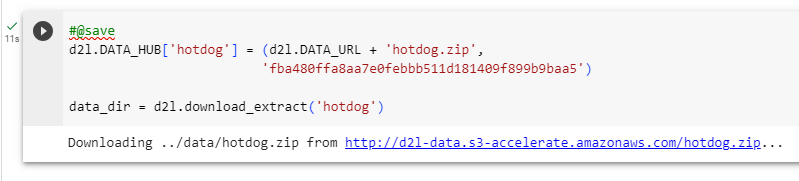
#@save
d2l.DATA_HUB['hotdog'] = (d2l.DATA_URL + 'hotdog.zip',
                         'fba480ffa8aa7e0febbb511d181409f899b9baa5')

data_dir = d2l.download_extract('hotdog')
이 코드는 D2L (Dive into Deep Learning) 라이브러리의 데이터 허브에 새로운 데이터셋을 등록하고 데이터셋을 다운로드하고 압축을 해제하는 역할을 합니다. 각 줄의 역할을 살펴보겠습니다:
- #@save: 이 주석은 코드 블록이 문서화를 위한 주석임을 나타냅니다. D2L에서는 이러한 주석을 사용하여 문서를 생성하는 데 활용합니다.
- d2l.DATA_HUB['hotdog'] = (d2l.DATA_URL + 'hotdog.zip', 'fba480ffa8aa7e0febbb511d181409f899b9baa5'): 이 줄은 데이터 허브에 'hotdog'라는 이름으로 새로운 데이터셋을 등록하는 역할을 합니다. 등록된 데이터셋에 대한 정보 (URL과 해시)를 제공합니다. 이 정보를 통해 데이터셋을 다운로드하고 검증할 수 있습니다.
- data_dir = d2l.download_extract('hotdog'): 이 코드는 등록한 'hotdog' 데이터셋을 다운로드하고 압축을 해제하여 로컬 디렉토리에 저장하는 역할을 합니다. 데이터셋의 다운로드 URL과 해시를 사용하여 데이터셋을 검증합니다. data_dir 변수에는 데이터셋이 저장된 로컬 디렉토리 경로가 저장됩니다.
이 코드 블록은 D2L 라이브러리의 데이터 허브에 새로운 데이터셋을 등록하고 해당 데이터셋을 다운로드하고 압축을 해제하여 사용할 수 있도록 준비하는 역할을 합니다.
Print number of images in the data_dir.
# Display the first 5 images
for i in range(5):
    img = mpimg.imread(image_files[i])
    plt.imshow(img)
    plt.axis('off')  # Turn off axis labels
    plt.show()
Number of images: 2800
We create two instances to read all the image files in the training and testing datasets, respectively.
교육 및 테스트 데이터 세트의 모든 이미지 파일을 읽기 위해 각각 두 개의 인스턴스를 만듭니다.
train_imgs = torchvision.datasets.ImageFolder(os.path.join(data_dir, 'train'))
test_imgs = torchvision.datasets.ImageFolder(os.path.join(data_dir, 'test'))
이 코드는 'hotdog' 데이터셋의 학습 및 테스트 이미지들을 로드하는 역할을 합니다. 이해하기 쉽게 코드를 분석해보겠습니다:
- #@save: 이 주석은 코드 블록이 문서화를 위한 주석임을 나타냅니다.
- train_imgs = torchvision.datasets.ImageFolder(os.path.join(data_dir, 'train')): 이 줄은 학습 이미지들이 포함된 디렉토리에서 이미지를 로드하여 train_imgs에 저장합니다. ImageFolder는 디렉토리 구조를 기반으로 이미지 데이터셋을 생성합니다. 학습 이미지들은 'train' 서브디렉토리에 저장되어 있습니다.
- test_imgs = torchvision.datasets.ImageFolder(os.path.join(data_dir, 'test')): 이 줄은 테스트 이미지들을 로드하여 test_imgs에 저장합니다. 테스트 이미지들은 'test' 서브디렉토리에 저장되어 있습니다.
이렇게 코드를 실행하면 'hotdog' 데이터셋의 학습 이미지와 테스트 이미지를 train_imgs와 test_imgs에 로드하게 됩니다. 'ImageFolder' 클래스는 데이터셋을 쉽게 관리하고 처리할 수 있도록 도와주는 유용한 도구입니다.
The first 8 positive examples and the last 8 negative images are shown below. As you can see, the images vary in size and aspect ratio.
처음 8개의 긍정적인 예와 마지막 8개의 부정적인 이미지가 아래에 나와 있습니다. 보시다시피 이미지의 크기와 종횡비가 다릅니다.
hotdogs = [train_imgs[i][0] for i in range(8)]
not_hotdogs = [train_imgs[-i - 1][0] for i in range(8)]
d2l.show_images(hotdogs + not_hotdogs, 2, 8, scale=1.4);
이 코드는 d2l (Dive into Deep Learning) 라이브러리의 d2l.show_images 함수를 사용하여 이미지 그리드를 표시하는 코드입니다. 이 함수는 이미지 목록을 격자 레이아웃으로 표시하는 데 사용됩니다.
코드의 각 부분이 하는 일은 다음과 같습니다.
- hotdogs = [train_imgs[i][0] for i in range(8)]: 이 줄은 train_imgs 데이터셋에서 처음 8개의 이미지를 담은 hotdogs 리스트를 생성합니다. hotdogs의 각 요소는 이미지를 나타내는 텐서입니다.
- not_hotdogs = [train_imgs[-i - 1][0] for i in range(8)]: 이 줄은 train_imgs 데이터셋에서 마지막 8개의 이미지를 담은 not_hotdogs 리스트를 생성합니다. 마찬가지로, not_hotdogs의 각 요소는 이미지를 나타내는 텐서입니다.
- d2l.show_images(hotdogs + not_hotdogs, 2, 8, scale=1.4);: 이 줄은 d2l.show_images 함수를 사용하여 이미지 그리드를 표시합니다. 표시할 이미지로 hotdogs와 not_hotdogs 리스트를 연결합니다. 2와 8 인자는 격자가 2행 8열을 가지도록 지정합니다. scale=1.4 인자는 표시되는 이미지의 크기를 조정하여 더 나은 가시성을 확보합니다.
요약하면, 이 코드는 d2l.show_images 함수를 사용하여 그리드 형태로 16개의 이미지를 표시합니다. 처음 8개 이미지는 핫도그이고, 마지막 8개 이미지는 핫도그가 아닌 이미지입니다.

During training, we first crop a random area of random size and random aspect ratio from the image, and then scale this area to a 224×224 input image. During testing, we scale both the height and width of an image to 256 pixels, and then crop a central 224×224 area as input. In addition, for the three RGB (red, green, and blue) color channels we standardize their values channel by channel. Concretely, the mean value of a channel is subtracted from each value of that channel and then the result is divided by the standard deviation of that channel.
학습하는 동안 먼저 이미지에서 임의의 크기와 가로 세로 비율의 임의 영역을 자른 다음 이 영역을 224×224 입력 이미지로 조정합니다. 테스트하는 동안 이미지의 높이와 너비를 모두 256픽셀로 조정한 다음 중앙 224×224 영역을 입력으로 자릅니다. 또한 3개의 RGB(빨간색, 녹색 및 파란색) 색상 채널의 경우 해당 값을 채널별로 표준화합니다. 구체적으로, 채널의 평균값을 해당 채널의 각 값에서 뺀 다음 결과를 해당 채널의 표준 편차로 나눕니다.
# Specify the means and standard deviations of the three RGB channels to
# standardize each channel
normalize = torchvision.transforms.Normalize(
    [0.485, 0.456, 0.406], [0.229, 0.224, 0.225])

train_augs = torchvision.transforms.Compose([
    torchvision.transforms.RandomResizedCrop(224),
    torchvision.transforms.RandomHorizontalFlip(),
    torchvision.transforms.ToTensor(),
    normalize])

test_augs = torchvision.transforms.Compose([
    torchvision.transforms.Resize([256, 256]),
    torchvision.transforms.CenterCrop(224),
    torchvision.transforms.ToTensor(),
    normalize])
이 코드는 이미지 데이터 전처리를 위한 변환들을 정의하는 부분입니다. 데이터셋을 학습 및 테스트용으로 나눈 후에, 각 데이터셋의 이미지에 대해 수행할 전처리 작업을 설정하는데 사용됩니다. 코드의 각 줄이 하는 역할을 살펴보겠습니다.
- normalize = torchvision.transforms.Normalize([0.485, 0.456, 0.406], [0.229, 0.224, 0.225]): 이 줄은 이미지 정규화를 위한 변환을 정의합니다. 정규화는 각 채널의 평균과 표준 편차를 사용하여 RGB 이미지를 정규화합니다. 이러한 정규화는 모델의 학습 안정성과 성능을 향상시키는 데 도움이 됩니다.
- train_augs = torchvision.transforms.Compose([...]): 이 줄은 학습 데이터에 적용할 전처리 과정을 정의합니다. torchvision.transforms.Compose 함수는 여러 개의 전처리 함수를 하나로 연결하여 적용할 수 있게 해줍니다. 학습 데이터에 적용되는 변환은 다음과 같습니다:
- RandomResizedCrop(224): 이미지를 임의의 크기로 자르고 224x224 크기로 크롭합니다.
- RandomHorizontalFlip(): 이미지를 수평으로 무작위로 뒤집습니다.
- ToTensor(): 이미지를 텐서 형식으로 변환합니다.
- normalize: 앞서 정의한 정규화를 적용합니다.
- test_augs = torchvision.transforms.Compose([...]): 이 줄은 테스트 데이터에 적용할 전처리 과정을 정의합니다. 테스트 데이터에 적용되는 변환은 다음과 같습니다:
- Resize([256, 256]): 이미지 크기를 256x256으로 조정합니다.
- CenterCrop(224): 이미지를 중앙을 기준으로 224x224 크기로 크롭합니다.
- ToTensor(): 이미지를 텐서 형식으로 변환합니다.
- normalize: 정규화를 적용합니다.
이렇게 정의된 train_augs와 test_augs는 학습 및 테스트 데이터셋에서 이미지에 적용될 전처리 변환들을 구성합니다.
14.2.2.2. Defining and Initializing the Model
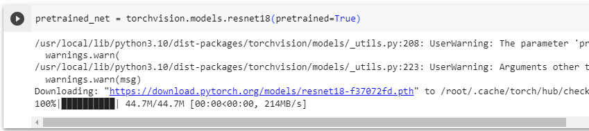
We use ResNet-18, which was pretrained on the ImageNet dataset, as the source model. Here, we specify pretrained=True to automatically download the pretrained model parameters. If this model is used for the first time, Internet connection is required for download.
ImageNet 데이터 세트에서 사전 훈련된 ResNet-18을 소스 모델로 사용합니다. 여기에서 pretrained=True를 지정하여 사전 훈련된 모델 매개변수를 자동으로 다운로드합니다. 이 모델을 처음 사용하는 경우 다운로드를 위해 인터넷 연결이 필요합니다.
pretrained_net = torchvision.models.resnet18(pretrained=True)이 코드는 torchvision 라이브러리의 resnet18 모델을 미리 학습된 가중치와 함께 불러오는 부분입니다.
torchvision.models.resnet18(pretrained=True)은 ResNet-18 아키텍처를 가져와서 미리 학습된 가중치를 사용하여 초기화한 모델을 생성합니다. ResNet-18은 18개의 층으로 구성된 딥 컨볼루션 신경망 아키텍처로, 이미지 분류와 같은 컴퓨터 비전 작업에서 널리 사용됩니다.
pretrained=True 매개변수는 미리 학습된 가중치를 사용하겠다는 의미입니다. 이렇게 하면 모델이 ImageNet 데이터셋에서 사전 학습된 가중치를 가져옵니다. ImageNet은 대규모 이미지 데이터셋으로, 다양한 카테고리에 속하는 이미지로 구성되어 있습니다. 이러한 사전 학습된 가중치는 초기화 단계에서 모델의 성능을 향상시키는 데 도움이 됩니다.
따라서 pretrained_net은 미리 학습된 ResNet-18 모델을 나타냅니다. 이 모델은 이미지 분류 작업에 사용될 수 있으며, 이미지 데이터를 입력으로 받아 각 클래스에 대한 확률 분포를 출력하는 역할을 할 수 있습니다.
사전 훈련된 소스 모델 인스턴스에는 여러 피처 레이어와 출력 레이어 fc가 포함되어 있습니다. 이 분할의 주요 목적은 출력 레이어를 제외한 모든 레이어의 모델 매개변수를 미세 조정하는 것입니다. 소스 모델의 멤버 변수 fc는 다음과 같습니다.
pretrained_net.fc
pretrained_net.fc는 미리 학습된 ResNet-18 모델의 마지막 fully connected (FC) 레이어를 나타냅니다.
ResNet-18 아키텍처의 마지막에는 fully connected 레이어가 존재하며, 이 레이어는 모델이 ImageNet 데이터셋과 같은 대규모 이미지 분류 작업에서 사용될 때 출력 클래스 수에 해당하는 뉴런을 가지고 있습니다. 이 fully connected 레이어는 이미지 특성을 활용하여 각 클래스에 대한 확률 분포를 생성합니다.
pretrained_net.fc를 호출하면 ResNet-18 모델의 마지막 fully connected 레이어가 반환됩니다. 이 레이어는 모델의 출력 역할을 하며, 이 레이어를 통과한 출력은 클래스 확률 분포를 나타냅니다. 이 fully connected 레이어를 변경하거나 새로운 데이터셋에 맞게 fine-tuning하는 등의 작업을 수행할 수 있습니다.

As a fully connected layer, it transforms ResNet’s final global average pooling outputs into 1000 class outputs of the ImageNet dataset. We then construct a new neural network as the target model. It is defined in the same way as the pretrained source model except that its number of outputs in the final layer is set to the number of classes in the target dataset (rather than 1000).
완전히 연결된 계층으로서 ResNet의 최종 글로벌 평균 풀링 출력을 ImageNet 데이터 세트의 1000개 클래스 출력으로 변환합니다. 그런 다음 대상 모델로 새로운 신경망을 구성합니다. 최종 계층의 출력 수가 대상 데이터 세트의 클래스 수(1000이 아닌)로 설정된다는 점을 제외하면 사전 훈련된 소스 모델과 동일한 방식으로 정의됩니다.
In the code below, the model parameters before the output layer of the target model instance finetune_net are initialized to model parameters of the corresponding layers from the source model. Since these model parameters were obtained via pretraining on ImageNet, they are effective. Therefore, we can only use a small learning rate to fine-tune such pretrained parameters. In contrast, model parameters in the output layer are randomly initialized and generally require a larger learning rate to be learned from scratch. Letting the base learning rate be η, a learning rate of 10η will be used to iterate the model parameters in the output layer.
η - eta
아래 코드에서 대상 모델 인스턴스 finetune_net의 출력 레이어 앞의 모델 매개변수는 소스 모델에서 해당 레이어의 모델 매개변수로 초기화됩니다. 이러한 모델 매개변수는 ImageNet에서 사전 학습을 통해 얻었기 때문에 효과적입니다. 따라서 사전 훈련된 매개변수를 미세 조정하기 위해 작은 학습 속도만 사용할 수 있습니다. 반대로 출력 계층의 모델 매개변수는 무작위로 초기화되며 일반적으로 처음부터 학습하려면 더 큰 학습률이 필요합니다. 기본 학습 속도를 η로 하면 출력 레이어에서 모델 매개변수를 반복하는 데 10η의 학습 속도가 사용됩니다.
finetune_net = torchvision.models.resnet18(pretrained=True)
finetune_net.fc = nn.Linear(finetune_net.fc.in_features, 2)
nn.init.xavier_uniform_(finetune_net.fc.weight);
위 코드는 미리 학습된 ResNet-18 아키텍처를 가져와서, 해당 아키텍처의 마지막 fully connected 레이어를 새로운 레이어로 교체하는 과정을 나타냅니다.
- finetune_net = torchvision.models.resnet18(pretrained=True): 미리 학습된 ResNet-18 모델을 가져옵니다. 이 모델은 ImageNet 데이터셋에서 학습되어 다양한 이미지 분류 작업에 사용할 수 있는 기본 아키텍처와 가중치를 가지고 있습니다.
- finetune_net.fc = nn.Linear(finetune_net.fc.in_features, 2): 기존의 마지막 fully connected 레이어를 새로운 선형 레이어로 교체합니다. 이 때, finetune_net.fc.in_features는 기존 fully connected 레이어의 입력 feature 수를 나타냅니다. 여기서는 이를 유지한 채로 출력 클래스 수를 2로 설정하여 이진 분류 작업에 적합하도록 모델을 수정합니다.
- nn.init.xavier_uniform_(finetune_net.fc.weight): 새로운 fully connected 레이어의 가중치를 Xavier 초기화 방법을 사용하여 초기화합니다. 이 초기화 방법은 신경망 가중치 초기화에 일반적으로 사용되는 방법 중 하나로, 초기 가중치를 효과적으로 설정해 네트워크의 학습을 원활하게 만듭니다.
이러한 수정 작업을 통해 ResNet-18 모델을 기존 분류 작업에서 새로운 이진 분류 작업에 맞게 fine-tuning할 수 있습니다. 새로운 fully connected 레이어는 2개의 클래스에 대한 확률 분포를 출력하도록 설정되어 이진 분류 작업을 수행할 수 있게 됩니다.
14.2.2.3. Fine-Tuning the Model
First, we define a training function train_fine_tuning that uses fine-tuning so it can be called multiple times.
먼저 여러 번 호출할 수 있도록 미세 조정을 사용하는 훈련 함수 train_fine_tuning을 정의합니다.
# If `param_group=True`, the model parameters in the output layer will be
# updated using a learning rate ten times greater
def train_fine_tuning(net, learning_rate, batch_size=128, num_epochs=5,
                      param_group=True):
    train_iter = torch.utils.data.DataLoader(torchvision.datasets.ImageFolder(
        os.path.join(data_dir, 'train'), transform=train_augs),
        batch_size=batch_size, shuffle=True)
    test_iter = torch.utils.data.DataLoader(torchvision.datasets.ImageFolder(
        os.path.join(data_dir, 'test'), transform=test_augs),
        batch_size=batch_size)
    devices = d2l.try_all_gpus()
    loss = nn.CrossEntropyLoss(reduction="none")
    if param_group:
        params_1x = [param for name, param in net.named_parameters()
             if name not in ["fc.weight", "fc.bias"]]
        trainer = torch.optim.SGD([{'params': params_1x},
                                   {'params': net.fc.parameters(),
                                    'lr': learning_rate * 10}],
                                lr=learning_rate, weight_decay=0.001)
    else:
        trainer = torch.optim.SGD(net.parameters(), lr=learning_rate,
                                  weight_decay=0.001)
    d2l.train_ch13(net, train_iter, test_iter, loss, trainer, num_epochs,
                   devices)
위 코드는 fine-tuning을 통해 사전 훈련된 신경망 모델을 새로운 작업에 맞게 학습시키는 과정을 정의한 함수를 나타냅니다.
- train_fine_tuning(net, learning_rate, batch_size=128, num_epochs=5, param_group=True): fine-tuning을 수행하기 위한 함수를 정의합니다. net은 모델, learning_rate는 학습률, batch_size는 배치 크기, num_epochs는 학습 에포크 수를 나타냅니다. param_group는 파라미터 그룹화 여부를 결정하는 매개변수로, True로 설정하면 출력 레이어의 가중치에 더 높은 학습률을 적용하는 방식을 사용합니다.
- train_iter와 test_iter: 학습 및 테스트 데이터를 DataLoader로 불러오는 과정을 나타냅니다. ImageFolder를 사용하여 데이터셋을 생성하고, transform을 통해 이미지 변환 작업을 수행합니다.
- devices = d2l.try_all_gpus(): 사용 가능한 GPU 디바이스를 모두 가져오는 과정입니다.
- loss = nn.CrossEntropyLoss(reduction="none"): 손실 함수를 교차 엔트로피 손실로 정의합니다. reduction을 "none"으로 설정하면 배치 내 각 샘플에 대한 손실 값을 구할 수 있습니다.
- if param_group:: param_group가 True인 경우, 모델 파라미터를 그룹화하여 학습률을 설정하는 방식을 사용합니다. 이 때, params_1x는 출력 레이어를 제외한 모든 파라미터를 가져오는 리스트입니다. 출력 레이어의 파라미터는 학습률을 10배로 높여서 적용합니다.
- trainer = torch.optim.SGD(...): SGD (stochastic gradient descent, 확률적 경사 하강법) 최적화 알고리즘을 사용하여 학습을 수행하는 옵티마이저를 정의합니다. params_1x와 출력 레이어의 파라미터에 서로 다른 학습률을 적용하도록 설정합니다.
- d2l.train_ch13(...): 정의한 학습 함수를 호출하여 fine-tuning 학습을 수행합니다. 학습과 테스트 데이터셋, 손실 함수, 옵티마이저 등을 인자로 전달하여 모델을 학습시킵니다.
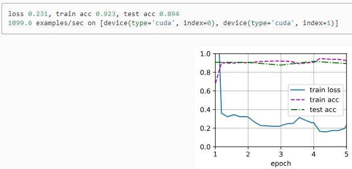
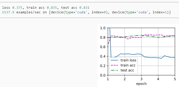
We set the base learning rate to a small value in order to fine-tune the model parameters obtained via pretraining. Based on the previous settings, we will train the output layer parameters of the target model from scratch using a learning rate ten times greater.
사전 학습을 통해 얻은 모델 매개 변수를 미세 조정하기 위해 기본 학습 속도를 작은 값으로 설정했습니다. 이전 설정을 기반으로 10배 더 큰 학습률을 사용하여 대상 모델의 출력 계층 매개변수를 처음부터 훈련합니다.
train_fine_tuning(finetune_net, 5e-5)위 코드는 fine-tuning을 통해 사전 훈련된 ResNet 모델인 finetune_net을 학습하는 과정을 나타냅니다.
- train_fine_tuning(finetune_net, 5e-5): train_fine_tuning 함수를 호출하여 finetune_net 모델을 학습합니다. 5e-5는 학습률을 나타내며, 여기서는 상대적으로 작은 학습률로 설정되어 있습니다. 따라서 finetune_net 모델을 학습하면서 학습률을 조절하여 새로운 작업에 맞게 가중치를 조정하게 됩니다.

For comparison, we define an identical model, but initialize all of its model parameters to random values. Since the entire model needs to be trained from scratch, we can use a larger learning rate.
비교를 위해 동일한 모델을 정의하지만 모든 모델 매개변수를 임의의 값으로 초기화합니다. 전체 모델을 처음부터 훈련해야 하므로 더 큰 학습률을 사용할 수 있습니다.
scratch_net = torchvision.models.resnet18()
scratch_net.fc = nn.Linear(scratch_net.fc.in_features, 2)
train_fine_tuning(scratch_net, 5e-4, param_group=False)
위 코드는 "from scratch"로 새로운 ResNet 모델을 생성하고 학습하는 과정을 나타냅니다.
- scratch_net = torchvision.models.resnet18(): 새로운 ResNet 모델을 생성합니다. 이 모델은 사전 훈련된 가중치 없이 초기화된 상태입니다.
- scratch_net.fc = nn.Linear(scratch_net.fc.in_features, 2): 생성한 새로운 ResNet 모델의 Fully Connected (FC) 레이어를 수정합니다. 입력 특성 개수에 따라 출력 특성 개수가 2인 FC 레이어로 변경됩니다. 이것은 분류 문제에서 두 개의 클래스를 구분하는 데 사용됩니다.
- train_fine_tuning(scratch_net, 5e-4, param_group=False): train_fine_tuning 함수를 호출하여 생성한 새로운 ResNet 모델 scratch_net을 학습합니다. 5e-4는 학습률을 나타내며, param_group=False로 설정되어 FC 레이어에 해당하는 가중치만 학습되며, 사전 훈련된 모델의 가중치는 고정됩니다. 이렇게 하면 새로운 작업에 맞게 FC 레이어만 학습됩니다.
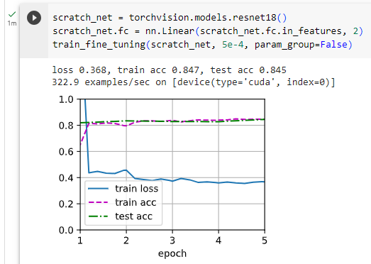
As we can see, the fine-tuned model tends to perform better for the same epoch because its initial parameter values are more effective.
보시다시피 미세 조정된 모델은 초기 매개변수 값이 더 효과적이기 때문에 동일한 에포크에 대해 더 나은 성능을 보이는 경향이 있습니다.
14.2.3. Summary
- Transfer learning transfers knowledge learned from the source dataset to the target dataset. Fine-tuning is a common technique for transfer learning.
전이 학습은 원본 데이터 세트에서 학습한 지식을 대상 데이터 세트로 이전합니다. 미세 조정은 전이 학습을 위한 일반적인 기술입니다. - The target model copies all model designs with their parameters from the source model except the output layer, and fine-tunes these parameters based on the target dataset. In contrast, the output layer of the target model needs to be trained from scratch.
대상 모델은 출력 레이어를 제외한 소스 모델의 매개변수가 있는 모든 모델 디자인을 복사하고 대상 데이터 세트를 기반으로 이러한 매개변수를 미세 조정합니다. 반대로 대상 모델의 출력 계층은 처음부터 학습해야 합니다. - Generally, fine-tuning parameters uses a smaller learning rate, while training the output layer from scratch can use a larger learning rate.
일반적으로 미세 조정 매개변수는 더 작은 학습률을 사용하는 반면 출력 계층을 처음부터 훈련하면 더 큰 학습률을 사용할 수 있습니다.
14.2.4. Exercises
- Keep increasing the learning rate of finetune_net. How does the accuracy of the model change?
- Further adjust hyperparameters of finetune_net and scratch_net in the comparative experiment. Do they still differ in accuracy?
- Set the parameters before the output layer of finetune_net to those of the source model and do not update them during training. How does the accuracy of the model change? You can use the following code.
for param in finetune_net.parameters():
    param.requires_grad = False
4. In fact, there is a “hotdog” class in the ImageNet dataset. Its corresponding weight parameter in the output layer can be obtained via the following code. How can we leverage this weight parameter?
weight = pretrained_net.fc.weight
hotdog_w = torch.split(weight.data, 1, dim=0)[934]
hotdog_w.shape
torch.Size([1, 512])'Dive into Deep Learning > D2L Computer Vision' 카테고리의 다른 글
| D2L - 14.10. Transposed Convolution (1) | 2023.08.21 |
|---|---|
| D2L - 14.9. Semantic Segmentation and the Dataset (0) | 2023.08.20 |
| D2L - 14.8. Region-based CNNs (R-CNNs) (0) | 2023.08.20 |
| D2L - 14.7. Single Shot Multibox Detection (0) | 2023.08.19 |
| D2L - 14.6. The Object Detection Dataset (0) | 2023.08.19 |
| D2L - 14.5. Multiscale Object Detection (0) | 2023.08.19 |
| D2L - 14.4. Anchor Boxes (0) | 2023.08.19 |
| D2L - 14.3. Object Detection and Bounding Boxes (0) | 2023.08.19 |
| D2L - 14.1. Image Augmentation (0) | 2023.08.19 |
| D2L - 14. Computer Vision (0) | 2023.08.18 |