

https://d2l.ai/chapter_computer-vision/image-augmentation.html
14.1. Image Augmentation — Dive into Deep Learning 1.0.0 documentation
d2l.ai
14.1. Image Augmentation
In Section 8.1, we mentioned that large datasets are a prerequisite for the success of deep neural networks in various applications. Image augmentation generates similar but distinct training examples after a series of random changes to the training images, thereby expanding the size of the training set. Alternatively, image augmentation can be motivated by the fact that random tweaks of training examples allow models to rely less on certain attributes, thereby improving their generalization ability. For example, we can crop an image in different ways to make the object of interest appear in different positions, thereby reducing the dependence of a model on the position of the object. We can also adjust factors such as brightness and color to reduce a model’s sensitivity to color. It is probably true that image augmentation was indispensable for the success of AlexNet at that time. In this section we will discuss this widely used technique in computer vision.
섹션 8.1에서 대규모 데이터 세트가 다양한 애플리케이션에서 심층 신경망의 성공을 위한 전제 조건이라고 언급했습니다. 이미지 확대는 트레이닝 이미지에 대한 일련의 무작위 변경 후에 유사하지만 별개의 트레이닝 예제를 생성하여 트레이닝 세트의 크기를 확장합니다. 또는 훈련 예제를 임의로 조정하면 모델이 특정 속성에 덜 의존하게 되므로 일반화 능력이 향상된다는 사실에 의해 이미지 확대가 동기가 될 수 있습니다. 예를 들어 관심 대상이 다른 위치에 나타나도록 다양한 방법으로 이미지를 잘라 대상 위치에 대한 모델의 의존성을 줄일 수 있습니다. 밝기 및 색상과 같은 요소를 조정하여 색상에 대한 모델의 민감도를 줄일 수도 있습니다. 당시 AlexNet의 성공을 위해 이미지 확대가 필수 불가결한 것은 아마도 사실일 것입니다. 이 섹션에서는 컴퓨터 비전에서 널리 사용되는 이 기술에 대해 설명합니다.
Image Augmentation이란?
Image augmentation refers to the process of applying various transformations to images in order to create new variations of the original images. This technique is commonly used in machine learning and computer vision tasks, especially in training deep learning models for image recognition, object detection, and other tasks. The goal of image augmentation is to increase the diversity and variability of the training dataset, which can lead to improved model generalization and performance on unseen data.
이미지 증강은 원본 이미지에 다양한 변환을 적용하여 새로운 변형된 이미지를 생성하는 과정을 말합니다. 이 기술은 주로 기계 학습과 컴퓨터 비전 작업에서 사용되며, 특히 이미지 인식, 물체 감지 및 기타 작업에 대한 딥 러닝 모델을 훈련할 때 많이 활용됩니다. 이미지 증강의 목표는 훈련 데이터셋의 다양성과 가변성을 증가시켜 모델의 일반화 성능과 새로운 데이터에서의 성능을 향상시키는 것입니다.
Image augmentation techniques involve making small, controlled changes to the images while preserving their semantic content. Some common image augmentation techniques include:
이미지 증강 기법은 이미지의 시맨틱 콘텐츠를 보존하면서 작은 제어된 변화를 가하는 것을 포함합니다. 일반적인 이미지 증강 기술로는 다음과 같은 것들이 있습니다:
- Horizontal and Vertical Flips: Mirroring the image horizontally or vertically to create variations.
수평 및 수직 뒤집기: 이미지를 수평 또는 수직으로 뒤집어서 변형을 만듭니다. - Rotation: Rotating the image by a certain degree.
회전: 이미지를 일정한 각도로 회전합니다. - Zoom: Enlarging or shrinking the image slightly.
확대 및 축소: 이미지를 약간 확대하거나 축소합니다. - Brightness and Contrast Adjustment: Changing the brightness and contrast levels of the image.
밝기 및 대비 조절: 이미지의 밝기와 대비 수준을 조정합니다. - Color Jittering: Applying small color changes to the image.
색상 조절: 이미지에 작은 색상 변화를 적용합니다. - Noise Addition: Adding small amounts of noise to the image.
노이즈 추가: 이미지에 작은 양의 노이즈를 추가합니다. - Random Cropping: Cropping a random portion of the image.
임의의 자르기: 이미지의 임의 부분을 자릅니다. - Elastic Transformations: Applying elastic deformations to the image.
탄성 변형: 이미지에 탄성 변형을 적용합니다.
These transformations help the model learn to be invariant to small changes in the input data, making it more robust and accurate when applied to real-world data.
이러한 변환은 모델이 입력 데이터의 작은 변화에 불변하게 학습하도록 도와줍니다. 이로써 모델은 실제 세계 데이터에 적용할 때 더 견고하고 정확하게 작동할 수 있게 됩니다.
In the context of deep learning and neural networks, image augmentation is often used during the training process to prevent overfitting, improve model generalization, and enhance the model's ability to handle various conditions and scenarios.
딥 러닝과 신경망의 맥락에서 이미지 증강image augmentation은 종종 훈련 과정 중에 사용되어 과적합을 방지하고 모델의 일반화 성능을 개선하며 다양한 조건과 시나리오를 처리할 수 있는 능력을 향상시킵니다.
%matplotlib inline
import torch
import torchvision
from torch import nn
from d2l import torch as d2l
14.1.1. Common Image Augmentation Methods
In our investigation of common image augmentation methods, we will use the following 400×500 image an example.
일반적인 이미지 확대 방법을 조사할 때 다음 400×500 이미지를 예로 사용합니다.
d2l.set_figsize()
img = d2l.Image.open('../img/cat1.jpg')
d2l.plt.imshow(img);

위 코드는 주피터 노트북에서 사용되는 코드로, 주어진 이미지 파일을 열어서 화면에 보여주는 예제입니다. 코드를 한 줄씩 살펴보겠습니다:
- %matplotlib inline: 이 라인은 주피터 노트북에서 그래프나 이미지 등을 인라인으로 표시하기 위한 명령입니다. 이를 통해 그래프나 이미지를 코드 셀 아래에 바로 표시할 수 있습니다.
- import torch: 파이토치 라이브러리를 가져옵니다.
- import torchvision: 파이토치의 torchvision 패키지를 가져옵니다. torchvision은 이미지 데이터셋 및 변환을 다루는 라이브러리입니다.
- from torch import nn: 파이토치의 nn 모듈에서 nn을 가져옵니다. nn은 신경망 모델을 구축하는 데 사용되는 모듈들을 포함하고 있습니다.
- from d2l import torch as d2l: d2l 라이브러리에서 torch 모듈을 가져와 d2l이라는 이름으로 사용합니다.
- d2l.set_figsize(): 그래프의 크기를 설정하는 d2l 라이브러리의 함수를 호출합니다.
- img = d2l.Image.open('../img/cat1.jpg'): d2l 라이브러리의 Image 모듈을 사용하여 '../img/cat1.jpg' 경로에 있는 이미지 파일을 엽니다. img 변수에 이미지 객체가 저장됩니다.
- d2l.plt.imshow(img): d2l 라이브러리의 plt 모듈을 사용하여 이미지를 표시합니다. imshow 함수를 호출하여 img를 표시하고, ;를 사용하여 출력 결과를 숨깁니다.
위 코드는 이미지 파일 '../img/cat1.jpg'를 열어서 주피터 노트북에서 화면에 표시하는 예제입니다. 이를 실행하면 해당 경로의 이미지가 출력되게 됩니다.
Most image augmentation methods have a certain degree of randomness. To make it easier for us to observe the effect of image augmentation, next we define an auxiliary function apply. This function runs the image augmentation method aug multiple times on the input image img and shows all the results.
대부분의 이미지 확대 image augmentation 방법에는 어느 정도의 무작위성이 있습니다. 이미지 확대 image augmentation 효과를 더 쉽게 관찰할 수 있도록 다음으로 보조 함수 적용을 정의합니다. 이 함수는 입력 이미지 img에서 이미지 확대 image augmentation 방법 aug를 여러 번 실행하고 모든 결과를 표시합니다.
def apply(img, aug, num_rows=2, num_cols=4, scale=1.5):
    Y = [aug(img) for _ in range(num_rows * num_cols)]
    d2l.show_images(Y, num_rows, num_cols, scale=scale)
위 코드는 이미지 변환 (Augmentation) 함수를 적용하여 변환된 이미지들을 그리드 형태로 표시하는 함수를 정의한 것입니다. 코드를 한 줄씩 살펴보겠습니다:
- def apply(img, aug, num_rows=2, num_cols=4, scale=1.5):: apply라는 함수를 정의합니다. 이 함수는 세 개의 인자를 받습니다. 첫 번째 인자 img는 입력 이미지입니다. 두 번째 인자 aug는 이미지 변환 함수를 나타냅니다. num_rows와 num_cols는 그리드에 표시할 행과 열의 개수를 지정하며, scale은 이미지의 크기를 조절하는 인자입니다.
- Y = [aug(img) for _ in range(num_rows * num_cols)]: aug 함수를 num_rows * num_cols번 반복하여 변환된 이미지들을 리스트 Y에 저장합니다. 각 반복마다 aug(img)를 호출하여 이미지를 변환합니다.
- d2l.show_images(Y, num_rows, num_cols, scale=scale): 변환된 이미지 리스트 Y를 num_rows 행과 num_cols 열로 나타내는 그리드 형태로 표시합니다. 이미지의 크기는 scale 인자를 사용하여 조절합니다.
즉, 위 함수 apply는 입력 이미지를 주어진 변환 함수로 여러 번 변환하여 그리드 형태로 출력하는 역할을 수행합니다. 이를 통해 이미지 변환의 효과를 시각적으로 확인할 수 있습니다.
14.1.1.1. Flipping and Cropping
Flipping the image left and right usually does not change the category of the object. This is one of the earliest and most widely used methods of image augmentation. Next, we use the transforms module to create the RandomHorizontalFlip instance, which flips an image left and right with a 50% chance.
이미지를 좌우로 뒤집는 것은 일반적으로 개체의 범주를 변경하지 않습니다. 이것은 이미지 확대의 가장 초기이자 가장 널리 사용되는 방법 중 하나입니다. 다음으로 변환transforms 모듈을 사용하여 이미지를 50%의 확률로 좌우로 뒤집는 RandomHorizontalFlip 인스턴스를 만듭니다.
apply(img, torchvision.transforms.RandomHorizontalFlip())
위 코드는 이미지 변환 함수를 적용하여 입력 이미지를 수평으로 뒤집은 후 변환된 이미지들을 그리드 형태로 표시하는 작업을 수행합니다. 코드를 한 줄씩 살펴보겠습니다:
- apply(img, torchvision.transforms.RandomHorizontalFlip()): apply 함수를 호출하여 입력 이미지 img에 torchvision.transforms.RandomHorizontalFlip() 변환 함수를 적용합니다. 이 변환 함수는 입력 이미지를 무작위로 수평으로 뒤집습니다. 즉, 이미지의 왼쪽과 오른쪽이 뒤바뀝니다.
위 코드는 apply 함수를 사용하여 입력 이미지를 수평으로 뒤집은 후 변환된 이미지들을 그리드 형태로 표시하는 작업을 수행합니다. 이를 통해 이미지 뒤집기 변환의 효과를 시각적으로 확인할 수 있습니다.
Flipping up and down is not as common as flipping left and right. But at least for this example image, flipping up and down does not hinder recognition. Next, we create a RandomVerticalFlip instance to flip an image up and down with a 50% chance.
위아래로 뒤집는 것은 좌우로 뒤집는 것만큼 일반적이지 않습니다. 그러나 적어도 이 예제 이미지의 경우 위아래로 뒤집는 것이 인식을 방해하지 않습니다. 다음으로 RandomVerticalFlip 인스턴스를 생성하여 50% 확률로 이미지를 위아래로 뒤집습니다.
apply(img, torchvision.transforms.RandomVerticalFlip())
위 코드는 입력 이미지에 수직으로 무작위로 뒤집기 변환을 적용하고, 이를 그리드 형태로 시각화하는 작업을 수행합니다. 코드를 단계별로 설명하겠습니다:
- apply(img, torchvision.transforms.RandomVerticalFlip()): apply 함수를 호출하여 입력 이미지 img에 torchvision.transforms.RandomVerticalFlip() 변환 함수를 적용합니다. 이 변환 함수는 입력 이미지를 무작위로 수직으로 뒤집습니다. 즉, 이미지의 위쪽과 아래쪽이 뒤바뀝니다.
이 코드는 입력 이미지를 수직으로 뒤집은 후 변환된 이미지들을 그리드 형태로 표시합니다. 이를 통해 이미지 뒤집기 변환의 효과를 시각적으로 확인할 수 있습니다.
In the example image we used, the cat is in the middle of the image, but this may not be the case in general. In Section 7.5, we explained that the pooling layer can reduce the sensitivity of a convolutional layer to the target position. In addition, we can also randomly crop the image to make objects appear in different positions in the image at different scales, which can also reduce the sensitivity of a model to the target position.
우리가 사용한 예제 이미지에서 고양이는 이미지 중앙에 있지만 일반적으로 그렇지 않을 수 있습니다. 7.5절에서 풀링 레이어가 목표 위치에 대한 컨볼루션 레이어의 민감도를 감소시킬 수 있다고 설명했습니다. 또한 이미지를 무작위로 잘라 개체가 이미지의 다른 위치에 다른 배율로 나타나도록 할 수도 있습니다. 이렇게 하면 대상 위치에 대한 모델의 민감도를 줄일 수도 있습니다.
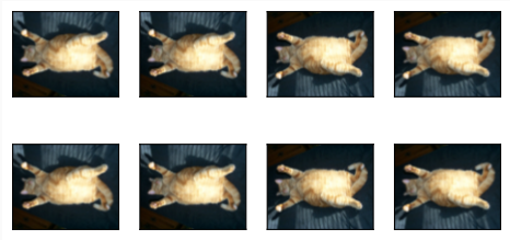
In the code below, we randomly crop an area with an area of 10%∼100% of the original area each time, and the ratio of width to height of this area is randomly selected from 0.5∼2. Then, the width and height of the region are both scaled to 200 pixels. Unless otherwise specified, the random number between a and b in this section refers to a continuous value obtained by random and uniform sampling from the interval [a,b].
아래 코드에서는 매번 원래 영역의 10%~100% 영역을 무작위로 자르고 이 영역의 너비와 높이의 비율을 0.5~2 중에서 무작위로 선택합니다. 그런 다음 영역의 너비와 높이가 모두 200픽셀로 조정됩니다. 달리 명시하지 않는 한, 이 섹션에서 a와 b 사이의 난수는 간격 [a,b]에서 무작위로 균일하게 샘플링하여 얻은 연속 값을 나타냅니다.
shape_aug = torchvision.transforms.RandomResizedCrop(
    (200, 200), scale=(0.1, 1), ratio=(0.5, 2))
apply(img, shape_aug)
위 코드는 입력 이미지에 무작위 크기와 종횡비로 자르기(resize crop) 변환을 적용하고, 이를 그리드 형태로 시각화하는 작업을 수행합니다. 코드를 단계별로 설명하겠습니다:
- shape_aug = torchvision.transforms.RandomResizedCrop((200, 200), scale=(0.1, 1), ratio=(0.5, 2)): torchvision.transforms.RandomResizedCrop() 변환 함수를 사용하여 shape_aug라는 변수에 무작위 크기로 자르기 변환을 생성합니다. 이 함수는 입력 이미지를 주어진 크기로 자르고, 무작위로 크기와 종횡비를 변화시킵니다. 여기서 (200, 200)은 자르고자 하는 크기를 의미하며, scale=(0.1, 1)은 무작위로 선택할 크기의 범위를 나타내고, ratio=(0.5, 2)는 무작위로 선택할 종횡비의 범위를 나타냅니다.
- apply(img, shape_aug): apply 함수를 호출하여 입력 이미지 img에 shape_aug로 정의된 변환 함수를 적용합니다. 이를 통해 입력 이미지에 무작위 크기와 종횡비로 자르기 변환을 적용한 이미지들을 그리드 형태로 표시합니다.
이 코드는 이미지를 무작위 크기와 종횡비로 자르는 변환을 적용하여 이미지의 다양한 부분을 추출하고 시각화하는 역할을 합니다.

14.1.1.2. Changing Colors
Another augmentation method is changing colors. We can change four aspects of the image color: brightness, contrast, saturation, and hue. In the example below, we randomly change the brightness of the image to a value between 50% (1−0.5) and 150% (1+0.5) of the original image.
또 다른 증강 방법은 색상을 변경하는 것입니다. 이미지 색상의 네 가지 측면인 밝기, 대비, 채도 및 색조를 변경할 수 있습니다. 아래 예에서는 이미지의 밝기를 원본 이미지의 50%(1−0.5)와 150%(1+0.5) 사이의 값으로 무작위로 변경합니다.
apply(img, torchvision.transforms.ColorJitter(
    brightness=0.5, contrast=0, saturation=0, hue=0))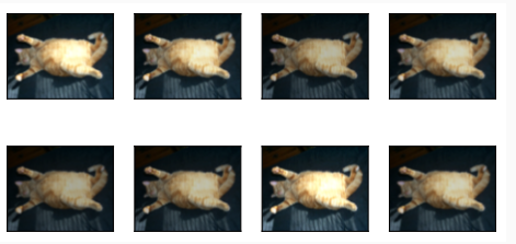
위 코드는 입력 이미지에 색상 조정 변환을 적용하고, 이를 시각화하는 작업을 수행합니다. 코드를 단계별로 설명하겠습니다:
- torchvision.transforms.ColorJitter(brightness=0.5, contrast=0, saturation=0, hue=0): torchvision.transforms.ColorJitter() 변환 함수를 사용하여 색상 조정 변환을 생성합니다. 이 함수는 입력 이미지의 색상을 조정하여 다양한 효과를 줄 수 있습니다. 여기서 brightness, contrast, saturation, hue 매개변수를 조정하여 각각 밝기, 대비, 채도, 색조를 조정할 수 있습니다. 각 매개변수의 값이 0보다 크면 변환이 적용됩니다.
- apply(img, torchvision.transforms.ColorJitter(brightness=0.5, contrast=0, saturation=0, hue=0)): apply 함수를 호출하여 입력 이미지 img에 색상 조정 변환 함수를 적용합니다. 이를 통해 입력 이미지에 다양한 색상 조정 효과를 적용한 이미지들을 그리드 형태로 표시합니다.
이 코드는 이미지의 색상을 다양하게 변화시켜 시각화하는 역할을 합니다. 여기서는 밝기를 조정하고 대비, 채도, 색조는 조정하지 않습니다.
Similarly, we can randomly change the hue of the image.
마찬가지로 이미지의 색조를 무작위로 변경할 수 있습니다.
apply(img, torchvision.transforms.ColorJitter(
    brightness=0, contrast=0, saturation=0, hue=0.5))

위 코드는 입력 이미지에 대한 torchvision.transforms.ColorJitter() 변환을 사용하여 색상 조정 변환을 적용하고, 이를 시각화하는 작업을 수행합니다. 코드를 단계별로 설명하겠습니다:
- torchvision.transforms.ColorJitter(brightness=0, contrast=0, saturation=0, hue=0.5): torchvision.transforms.ColorJitter() 변환 함수를 사용하여 색상 조정 변환을 생성합니다. 여기서 brightness, contrast, saturation 매개변수를 0으로 설정하고, hue 매개변수를 0.5로 설정하여 색조에 대한 조정만 적용될 수 있도록 합니다. hue 값이 0.5이므로 이미지의 색조가 최대 ±0.5만큼 변경됩니다.
- apply(img, torchvision.transforms.ColorJitter(brightness=0, contrast=0, saturation=0, hue=0.5)): apply 함수를 호출하여 입력 이미지 img에 색상 조정 변환 함수를 적용합니다. 이를 통해 입력 이미지에 다양한 색조 조정 효과를 적용한 이미지들을 그리드 형태로 표시합니다.
이 코드는 이미지의 색조를 다양하게 변화시켜 시각화하는 역할을 합니다.
We can also create a RandomColorJitter instance and set how to randomly change the brightness, contrast, saturation, and hue of the image at the same time.
또한 RandomColorJitter 인스턴스를 생성하고 동시에 이미지의 밝기, 대비, 채도 및 색조를 무작위로 변경하는 방법을 설정할 수 있습니다.
color_aug = torchvision.transforms.ColorJitter(
    brightness=0.5, contrast=0.5, saturation=0.5, hue=0.5)
apply(img, color_aug)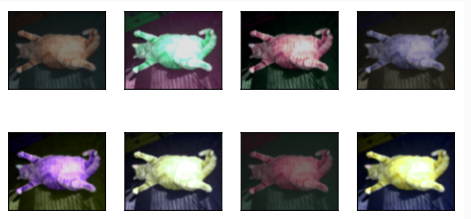
위 코드는 torchvision.transforms.ColorJitter() 변환을 사용하여 입력 이미지에 다양한 색상 조정을 적용하고, 이를 시각화하는 작업을 수행합니다. 코드를 단계별로 설명하겠습니다:
- torchvision.transforms.ColorJitter(brightness=0.5, contrast=0.5, saturation=0.5, hue=0.5): torchvision.transforms.ColorJitter() 변환 함수를 사용하여 색상 조정 변환을 생성합니다. 여기서 brightness, contrast, saturation 매개변수를 0.5로 설정하고, hue 매개변수를 0.5로 설정하여 밝기, 대비, 채도, 색조에 대한 조정을 적용할 수 있도록 합니다. 이렇게 설정하면 입력 이미지의 색상이 다양하게 변화됩니다.
- apply(img, color_aug): apply 함수를 호출하여 입력 이미지 img에 색상 조정 변환 함수 color_aug를 적용합니다. 이를 통해 입력 이미지에 다양한 색상 조정 효과를 적용한 이미지들을 그리드 형태로 표시합니다.
이 코드는 입력 이미지의 밝기, 대비, 채도, 색조를 다양하게 변화시켜 시각화하는 역할을 합니다.
14.1.1.3. Combining Multiple Image Augmentation Methods
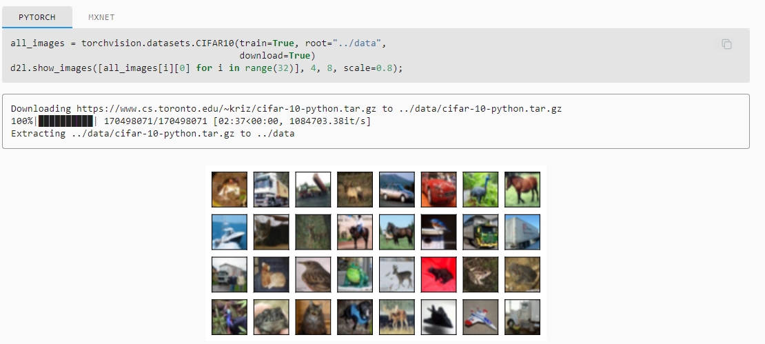
In practice, we will combine multiple image augmentation methods. For example, we can combine the different image augmentation methods defined above and apply them to each image via a Compose instance.
실제로는 여러 이미지 확대 방법을 결합합니다. 예를 들어 위에서 정의한 다양한 이미지 확대 방법을 결합하고 Compose 인스턴스를 통해 각 이미지에 적용할 수 있습니다.
all_images = torchvision.datasets.CIFAR10(train=True, root="../data",
                                          download=True)
d2l.show_images([all_images[i][0] for i in range(32)], 4, 8, scale=0.8);
위 코드는 CIFAR-10 데이터셋에서 이미지를 가져와 시각화하는 작업을 수행합니다. 코드를 단계별로 설명하겠습니다:
- torchvision.datasets.CIFAR10(train=True, root="../data", download=True): CIFAR-10 데이터셋을 로드합니다. train 매개변수를 True로 설정하여 학습 데이터셋을 로드하며, root 매개변수에 데이터의 저장 경로를 지정합니다. download 매개변수를 True로 설정하면 데이터셋을 다운로드합니다.
- [all_images[i][0] for i in range(32)]: CIFAR-10 데이터셋에서 처음부터 32개의 이미지를 가져와 리스트로 만듭니다. 각 이미지 데이터는 (이미지, 레이블) 형태로 저장되어 있으며, 여기서는 이미지 데이터만을 선택합니다.
- d2l.show_images([...], 4, 8, scale=0.8): d2l.show_images() 함수를 사용하여 이미지 리스트를 그리드 형태로 시각화합니다. 4는 그리드의 행 수, 8은 그리드의 열 수를 나타냅니다. scale 매개변수는 이미지 크기의 스케일을 조절하는 역할을 합니다.
이 코드는 CIFAR-10 데이터셋에서 가져온 처음 32개의 이미지를 4x8 그리드로 시각화하여 보여줍니다.
In order to obtain definitive results during prediction, we usually only apply image augmentation to training examples, and do not use image augmentation with random operations during prediction. Here we only use the simplest random left-right flipping method. In addition, we use a ToTensor instance to convert a minibatch of images into the format required by the deep learning framework, i.e., 32-bit floating point numbers between 0 and 1 with the shape of (batch size, number of channels, height, width).
예측 중에 결정적인 결과를 얻기 위해 일반적으로 훈련 예제에만 이미지 확대를 적용하고 예측 중에 임의 작업으로 이미지 확대를 사용하지 않습니다. 여기서는 가장 간단한 임의의 좌우 뒤집기 방법만 사용합니다. 또한 ToTensor 인스턴스를 사용하여 이미지의 미니 배치를 딥 러닝 프레임워크에 필요한 형식, 즉 (배치 크기, 채널 수, 높이, 너비).
train_augs = torchvision.transforms.Compose([
     torchvision.transforms.RandomHorizontalFlip(),
     torchvision.transforms.ToTensor()])

test_augs = torchvision.transforms.Compose([
     torchvision.transforms.ToTensor()])
위 코드는 데이터 증강을 위한 데이터 변환 함수들을 정의하는 작업을 수행합니다. 코드를 단계별로 설명하겠습니다:
- train_augs: 학습 데이터에 적용할 데이터 증강 변환 함수들을 조합한 객체를 생성합니다. torchvision.transforms.Compose() 함수를 사용하여 여러 변환 함수들을 순차적으로 적용할 수 있습니다.
- torchvision.transforms.RandomHorizontalFlip(): 무작위로 이미지를 수평으로 뒤집는 데이터 증강을 수행합니다. 이는 이미지를 좌우로 반전시키는 효과를 줍니다.
- torchvision.transforms.ToTensor(): 이미지를 텐서 형태로 변환합니다. 이 작업은 이미지 데이터를 신경망에 입력하기 위해 필요한 전처리 단계 중 하나입니다.
- test_augs: 테스트 데이터에 적용할 데이터 변환 함수들을 조합한 객체를 생성합니다. 여기서는 테스트 데이터에는 이미지 뒤집기 등의 변환을 적용하지 않고, 단순히 이미지를 텐서로 변환하는 ToTensor() 변환만 적용합니다.
이렇게 정의된 train_augs와 test_augs 객체는 학습 및 테스트 데이터에 데이터 증강 및 전처리를 적용할 때 사용됩니다. 학습 데이터에는 수평 뒤집기와 이미지를 텐서로 변환하는 작업이 수행되며, 테스트 데이터에는 이미지를 텐서로 변환하는 작업만 수행됩니다.
Next, we define an auxiliary function to facilitate reading the image and applying image augmentation. The transform argument provided by PyTorch’s dataset applies augmentation to transform the images. For a detailed introduction to DataLoader, please refer to Section 4.2.
다음으로 이미지 읽기 및 이미지 확대 적용을 용이하게 하는 보조 기능을 정의합니다. PyTorch의 데이터 세트에서 제공하는 변환 인수는 증강을 적용하여 이미지를 변환합니다. DataLoader에 대한 자세한 소개는 섹션 4.2를 참조하십시오.
def load_cifar10(is_train, augs, batch_size):
    dataset = torchvision.datasets.CIFAR10(root="../data", train=is_train,
                                           transform=augs, download=True)
    dataloader = torch.utils.data.DataLoader(dataset, batch_size=batch_size,
                    shuffle=is_train, num_workers=d2l.get_dataloader_workers())
    return dataloader
위 코드는 CIFAR-10 데이터셋을 로드하는 함수인 load_cifar10를 정의하는 부분입니다. 코드를 단계별로 설명하겠습니다:
- is_train: 학습 데이터인지 테스트 데이터인지를 나타내는 인자입니다. True이면 학습 데이터를, False이면 테스트 데이터를 로드합니다.
- augs: 데이터 증강 및 전처리를 적용하기 위한 데이터 변환 함수를 받는 인자입니다. 앞서 정의한 train_augs 또는 test_augs와 같은 변환 함수 객체를 여기에 전달합니다.
- batch_size: 배치 크기를 나타내는 인자입니다. 데이터를 미니배치로 나눠서 로드할 때 한 번에 로드되는 데이터 샘플의 개수입니다.
- torchvision.datasets.CIFAR10(): CIFAR-10 데이터셋을 로드하는 함수입니다. 해당 데이터셋은 지정된 경로에서 이미 다운로드된 경우 로드하며, 그렇지 않은 경우 다운로드합니다. 데이터셋은 CIFAR-10의 학습 데이터 또는 테스트 데이터 중 하나를 선택하여 로드합니다.
- transform: 데이터 변환 함수 객체를 전달합니다. 이를 통해 데이터 증강 및 전처리 작업을 수행합니다.
- torch.utils.data.DataLoader(): 데이터셋을 미니배치 형태로 로드하기 위한 데이터 로더 객체를 생성합니다. 배치 크기와 데이터 순서를 지정하여 데이터를 로드하며, 필요한 경우 데이터 로드를 병렬화합니다.
- d2l.get_dataloader_workers(): 데이터 로더를 병렬화할 때 사용할 워커의 수를 반환하는 함수입니다. 데이터 로드 성능을 향상시키기 위해 병렬 처리에 사용됩니다.
- 반환값: 로드된 데이터셋을 배치 단위로 로드하는 데이터 로더 객체를 반환합니다. 이를 통해 학습 또는 테스트 데이터를 미니배치 형태로 반복해서 사용할 수 있습니다.
14.1.2.1. Multi-GPU Training
#@save
def train_batch_ch13(net, X, y, loss, trainer, devices):
    """Train for a minibatch with multiple GPUs (defined in Chapter 13)."""
    if isinstance(X, list):
        # Required for BERT fine-tuning (to be covered later)
        X = [x.to(devices[0]) for x in X]
    else:
        X = X.to(devices[0])
    y = y.to(devices[0])
    net.train()
    trainer.zero_grad()
    pred = net(X)
    l = loss(pred, y)
    l.sum().backward()
    trainer.step()
    train_loss_sum = l.sum()
    train_acc_sum = d2l.accuracy(pred, y)
    return train_loss_sum, train_acc_sum

#@save
def train_ch13(net, train_iter, test_iter, loss, trainer, num_epochs,
               devices=d2l.try_all_gpus()):
    """Train a model with multiple GPUs (defined in Chapter 13)."""
    timer, num_batches = d2l.Timer(), len(train_iter)
    animator = d2l.Animator(xlabel='epoch', xlim=[1, num_epochs], ylim=[0, 1],
                            legend=['train loss', 'train acc', 'test acc'])
    net = nn.DataParallel(net, device_ids=devices).to(devices[0])
    for epoch in range(num_epochs):
        # Sum of training loss, sum of training accuracy, no. of examples,
        # no. of predictions
        metric = d2l.Accumulator(4)
        for i, (features, labels) in enumerate(train_iter):
            timer.start()
            l, acc = train_batch_ch13(
                net, features, labels, loss, trainer, devices)
            metric.add(l, acc, labels.shape[0], labels.numel())
            timer.stop()
            if (i + 1) % (num_batches // 5) == 0 or i == num_batches - 1:
                animator.add(epoch + (i + 1) / num_batches,
                             (metric[0] / metric[2], metric[1] / metric[3],
                              None))
        test_acc = d2l.evaluate_accuracy_gpu(net, test_iter)
        animator.add(epoch + 1, (None, None, test_acc))
    print(f'loss {metric[0] / metric[2]:.3f}, train acc '
          f'{metric[1] / metric[3]:.3f}, test acc {test_acc:.3f}')
    print(f'{metric[2] * num_epochs / timer.sum():.1f} examples/sec on '
          f'{str(devices)}')
위 코드는 다중 GPU를 활용하여 모델을 학습하는 함수인 train_ch13와 해당 함수 내에서 호출되는 train_batch_ch13 함수를 정의하는 부분입니다. 코드를 단계별로 설명하겠습니다:
- train_batch_ch13(net, X, y, loss, trainer, devices): 다중 GPU로 미니배치 학습을 수행하는 함수입니다. 인자로는 모델 net, 입력 데이터 X, 레이블 데이터 y, 손실 함수 loss, 옵티마이저 trainer, 그리고 사용할 GPU 디바이스들의 리스트 devices가 전달됩니다. 이 함수는 미니배치를 처리하고, 손실 계산, 역전파, 가중치 갱신 등의 학습 과정을 수행합니다.
- train_ch13(net, train_iter, test_iter, loss, trainer, num_epochs, devices=d2l.try_all_gpus()): 다중 GPU로 모델을 학습하는 함수입니다. 인자로는 모델 net, 학습 데이터 로더 train_iter, 테스트 데이터 로더 test_iter, 손실 함수 loss, 옵티마이저 trainer, 학습 에포크 수 num_epochs, 그리고 사용할 GPU 디바이스들의 리스트 devices가 전달됩니다. 이 함수는 각 에포크마다 학습과 평가 과정을 반복하여 모델을 학습하고 성능을 평가합니다.
- nn.DataParallel(net, device_ids=devices).to(devices[0]): DataParallel을 사용하여 모델 net을 여러 GPU에 병렬화하여 할당하는 과정입니다. 병렬화된 모델은 devices[0]에 할당됩니다.
- d2l.Accumulator(4): 성능 메트릭을 누적하기 위한 Accumulator 객체를 생성합니다. 누적할 값은 손실, 정확도, 데이터 샘플 수, 예측 수로 총 4개입니다.
- timer.start() 및 timer.stop(): 각 미니배치 학습 시간을 측정하기 위한 타이머를 시작하고 중지합니다.
- d2l.evaluate_accuracy_gpu(net, test_iter): 테스트 데이터에 대한 정확도를 GPU를 이용하여 평가하는 함수입니다.
- animator.add(...): 학습 과정 및 성능 변화를 시각화하는 Animator 객체에 정보를 추가합니다.
- 마지막에는 각 에포크마다 학습 및 평가 결과를 출력하고, 처리한 예제 수에 대한 처리 속도도 출력합니다.
이러한 함수를 사용하면 다중 GPU를 활용하여 모델을 학습하고 성능을 평가할 수 있습니다.
Now we can define the train_with_data_aug function to train the model with image augmentation. This function gets all available GPUs, uses Adam as the optimization algorithm, applies image augmentation to the training dataset, and finally calls the train_ch13 function just defined to train and evaluate the model.
이제 train_with_data_aug 함수를 정의하여 이미지 확대image augmentation로 모델을 훈련할 수 있습니다. 이 함수는 사용 가능한 모든 GPU를 가져오고 Adam을 최적화 알고리즘으로 사용하며 훈련 데이터 세트에 이미지 증대를 적용하고 마지막으로 방금 정의한 train_ch13 함수를 호출하여 모델을 훈련하고 평가합니다.
batch_size, devices, net = 256, d2l.try_all_gpus(), d2l.resnet18(10, 3)
net.apply(d2l.init_cnn)

def train_with_data_aug(train_augs, test_augs, net, lr=0.001):
    train_iter = load_cifar10(True, train_augs, batch_size)
    test_iter = load_cifar10(False, test_augs, batch_size)
    loss = nn.CrossEntropyLoss(reduction="none")
    trainer = torch.optim.Adam(net.parameters(), lr=lr)
    net(next(iter(train_iter))[0])
    train_ch13(net, train_iter, test_iter, loss, trainer, 10, devices)
위 코드는 데이터 증강을 적용하여 ResNet-18 모델을 학습하는 과정을 정의하는 부분입니다. 코드를 단계별로 설명하겠습니다:
- batch_size, devices, net: 미니배치 크기 batch_size, 사용 가능한 GPU 디바이스 리스트 devices, 그리고 d2l.resnet18 함수를 사용하여 클래스 수 10개, 입력 채널 3개인 ResNet-18 모델 net을 생성합니다.
- net.apply(d2l.init_cnn): 모델의 가중치 초기화를 위해 d2l.init_cnn 함수를 적용합니다. 이 함수는 모델 내부의 합성곱 레이어의 가중치를 초기화합니다.
- train_with_data_aug(train_augs, test_augs, net, lr=0.001): 데이터 증강을 적용하여 모델을 학습하는 함수입니다. 인자로는 학습 데이터 증강 변환 train_augs, 테스트 데이터 증강 변환 test_augs, 모델 net, 학습률 lr이 전달됩니다. 이 함수는 데이터 로더를 생성하고, 손실 함수, 옵티마이저 등을 설정하여 모델을 학습합니다.
- train_iter = load_cifar10(True, train_augs, batch_size): 학습 데이터 로더를 생성합니다. load_cifar10 함수를 사용하여 CIFAR-10 학습 데이터에 데이터 증강을 적용한 후 미니배치 크기 batch_size로 분할합니다.
- test_iter = load_cifar10(False, test_augs, batch_size): 테스트 데이터 로더를 생성합니다. 학습 데이터와 마찬가지로 테스트 데이터에 데이터 증강을 적용하고 미니배치 크기 batch_size로 분할합니다.
- loss = nn.CrossEntropyLoss(reduction="none"): 손실 함수로 교차 엔트로피 손실 함수를 사용하며, reduction 인자를 "none"으로 설정하여 각 샘플에 대한 손실 값을 반환합니다.
- trainer = torch.optim.Adam(net.parameters(), lr=lr): Adam 옵티마이저를 생성하고, 모델의 파라미터를 최적화 대상으로 설정합니다. 학습률은 lr로 설정됩니다.
- net(next(iter(train_iter))[0]): 모델의 가중치를 초기화하고, 모델의 출력을 계산하여 GPU 메모리에 모델을 적재합니다.
- train_ch13(net, train_iter, test_iter, loss, trainer, 10, devices): 다중 GPU를 활용하여 모델을 학습하는 train_ch13 함수를 호출하여 모델을 학습하고 성능을 평가합니다. 학습과 평가는 각각 10 에포크 동안 수행됩니다.
이러한 과정을 통해 데이터 증강을 적용하고, ResNet-18 모델을 학습하며 성능을 평가하는 과정이 구현되어 있습니다.
Let’s train the model using image augmentation based on random left-right flipping.
무작위 좌우 반전을 기반으로 한 이미지 확대를 사용하여 모델을 훈련시켜 봅시다.
train_with_data_aug(train_augs, test_augs, net)
14.1.3. Summary
- Image augmentation generates random images based on existing training data to improve the generalization ability of models.
이미지 증대는 모델의 일반화 능력을 향상시키기 위해 기존 학습 데이터를 기반으로 임의의 이미지를 생성합니다. - In order to obtain definitive results during prediction, we usually only apply image augmentation to training examples, and do not use image augmentation with random operations during prediction.
예측 중에 결정적인 결과를 얻기 위해 일반적으로 훈련 예제에만 이미지 확대를 적용하고 예측 중에 임의 작업으로 이미지 확대를 사용하지 않습니다. - Deep learning frameworks provide many different image augmentation methods, which can be applied simultaneously.
딥 러닝 프레임워크는 동시에 적용할 수 있는 다양한 이미지 확대 image augmentation 방법을 제공합니다.
14.1.4. Exercises
- Train the model without using image augmentation: train_with_data_aug(test_augs, test_augs). Compare training and testing accuracy when using and not using image augmentation. Can this comparative experiment support the argument that image augmentation can mitigate overfitting? Why?
- Combine multiple different image augmentation methods in model training on the CIFAR-10 dataset. Does it improve test accuracy?
- Refer to the online documentation of the deep learning framework. What other image augmentation methods does it also provide?
'Dive into Deep Learning > D2L Computer Vision' 카테고리의 다른 글
| D2L - 14.10. Transposed Convolution (1) | 2023.08.21 |
|---|---|
| D2L - 14.9. Semantic Segmentation and the Dataset (0) | 2023.08.20 |
| D2L - 14.8. Region-based CNNs (R-CNNs) (0) | 2023.08.20 |
| D2L - 14.7. Single Shot Multibox Detection (0) | 2023.08.19 |
| D2L - 14.6. The Object Detection Dataset (0) | 2023.08.19 |
| D2L - 14.5. Multiscale Object Detection (0) | 2023.08.19 |
| D2L - 14.4. Anchor Boxes (0) | 2023.08.19 |
| D2L - 14.3. Object Detection and Bounding Boxes (0) | 2023.08.19 |
| D2L - 14.2. Fine-Tuning (0) | 2023.08.19 |
| D2L - 14. Computer Vision (0) | 2023.08.18 |