
D2L - 14.10. Transposed Convolution
2023. 8. 21. 01:26 |
https://d2l.ai/chapter_computer-vision/transposed-conv.html
14.10. Transposed Convolution — Dive into Deep Learning 1.0.3 documentation
d2l.ai
14.10. Transposed Convolution
The CNN layers we have seen so far, such as convolutional layers (Section 7.2) and pooling layers (Section 7.5), typically reduce (downsample) the spatial dimensions (height and width) of the input, or keep them unchanged. In semantic segmentation that classifies at pixel-level, it will be convenient if the spatial dimensions of the input and output are the same. For example, the channel dimension at one output pixel can hold the classification results for the input pixel at the same spatial position.
우리가 지금까지 본 컨볼루션 레이어(섹션 7.2) 및 풀링 레이어(섹션 7.5)와 같은 CNN 레이어는 일반적으로 입력의 공간 차원 spatial dimensions (높이 및 너비)을 줄이거나 변경하지 않고 유지합니다. 픽셀 단위로 분류하는 시맨틱 분할semantic segmentation에서는 입력과 출력의 공간적 차원이 같으면 편리할 것이다. 예를 들어, 한 출력 픽셀의 채널 차원은 동일한 공간 위치에서 입력 픽셀에 대한 분류 결과를 보유할 수 있습니다.
To achieve this, especially after the spatial dimensions are reduced by CNN layers, we can use another type of CNN layers that can increase (upsample) the spatial dimensions of intermediate feature maps. In this section, we will introduce transposed convolution, which is also called fractionally-strided convolution (Dumoulin and Visin, 2016), for reversing downsampling operations by the convolution.
이를 달성하기 위해 특히 공간 차원이 CNN 레이어에 의해 축소된 후 중간 피쳐 맵의 공간 차원을 증가(업샘플링)할 수 있는 다른 유형의 CNN 레이어를 사용할 수 있습니다. 이 섹션에서는 convolution에 의한 downsampling 연산을 반전시키기 위해 fractionally-strided convolution(Dumoulin and Visin, 2016)이라고도 하는 transposed convolution을 소개합니다.
import torch
from torch import nn
from d2l import torch as d2l
Transposed Convolution이란?
Transposed convolution, also known as fractionally strided convolution or deconvolution, is an operation in convolutional neural networks (CNNs) that performs an upscaling operation on an input feature map. Unlike regular convolution, which reduces the spatial resolution of the feature map, transposed convolution increases the spatial resolution of the feature map.
전치 합성곱(Transposed Convolution), 또는 분수 합성곱 또는 역 합성곱(deconvolution)으로도 알려져 있으며, 컨볼루션 신경망(CNN)에서 입력 특성 맵에 대한 업스케일링 작업을 수행하는 연산입니다. 일반적인 컨볼루션과는 달리, 전치 합성곱은 특성 맵의 공간 해상도를 증가시킵니다.
The operation involves using learnable parameters (also known as convolutional kernels) to map each input pixel to multiple output pixels. This process effectively enlarges the feature map by inserting zeros or duplicating values in between the original input values. Transposed convolution is commonly used for tasks like image segmentation, image generation, and increasing the spatial resolution of feature maps.
이 연산은 학습 가능한 매개변수(컨볼루션 커널이라고도 함)를 사용하여 각 입력 픽셀을 여러 출력 픽셀로 매핑합니다. 이 과정은 원래 입력 값 사이에 0을 삽입하거나 값을 복제하여 특성 맵을 확장합니다. 전치 합성곱은 이미지 세그멘테이션, 이미지 생성, 특성 맵의 공간 해상도 증가와 같은 작업에 널리 사용됩니다.
The main steps of the transposed convolution operation are as follows:
전치 합성곱 연산의 주요 단계는 다음과 같습니다:
- Input: The input feature map has a certain height and width, and it is commonly represented as a 3D tensor with dimensions (channels, height, width).
입력: 입력 특성 맵은 특정한 높이와 너비를 갖고 있으며, 보통 (채널, 높이, 너비) 차원의 3D 텐서로 나타납니다. - Convolution: A set of learnable convolutional kernels (filters) is applied to the input feature map. Each kernel produces a response map by convolving with the input.
컨볼루션: 학습 가능한 컨볼루션 커널(필터) 집합이 입력 특성 맵에 적용됩니다. 각 커널은 입력과 컨볼루션하여 응답 맵을 생성합니다. - Upsampling: The response maps are then upsampled to increase the spatial resolution. This is achieved by inserting zeros or duplicating values in between the original input values, effectively increasing the size of the feature map.
업스케일링: 응답 맵은 업스케일링되어 공간 해상도를 증가시킵니다. 이를 위해 원래 입력 값 사이에 0을 삽입하거나 값을 복제하여 특성 맵의 크기를 키웁니다. - Output: The final output is an upsampled feature map with higher spatial resolution, which can be used for subsequent tasks like segmentation or generating higher-resolution images.
출력: 최종 출력은 공간 해상도가 높아진 업스케일링된 특성 맵으로, 세그멘테이션이나 더 높은 해상도의 이미지 생성과 같은 후속 작업에 사용할 수 있습니다.
Transposed convolution is commonly used in various architectures, such as in generative adversarial networks (GANs) for image generation and in decoder portions of autoencoders for feature reconstruction. It provides a way to recover spatial information that might have been lost during earlier convolutional operations, enabling the network to generate fine-grained details and high-resolution representations.
전치 합성곱은 이미지 생성을 위한 생성적 적대 신경망(GAN)이나 특성 재구성을 위한 오토인코더의 디코더 부분과 같은 다양한 아키텍처에서 자주 사용됩니다. 이를 통해 네트워크는 이전 컨볼루션 연산 중에 손실될 수 있는 공간 정보를 복구하여 미세한 세부 정보와 고해상도 표현을 생성할 수 있는 방법을 제공 합니다.
GAN이란 ?
GAN stands for "Generative Adversarial Network." It is a class of machine learning models that consists of two neural networks, known as the generator and the discriminator, that are trained simultaneously through a competitive process.
The key idea behind GANs is to have two networks compete against each other in a game-like scenario:
GAN은 "생성적 적대 신경망"을 의미합니다. 이는 생성자(generator)와 판별자(discriminator) 두 개의 신경망으로 구성되어 있으며, 이들이 경쟁적인 과정을 통해 동시에 훈련되는 머신 러닝 모델의 한 유형입니다.
GAN의 핵심 아이디어는 두 개의 신경망을 게임과 유사한 상황에서 서로 경쟁하게 하는 것입니다:
- Generator: The generator network takes random noise as input and generates data, such as images, audio, or text. It learns to create data that is similar to real data from a given dataset.
생성자: 생성자 신경망은 무작위한 잡음을 입력으로 받아 이미지, 음성 또는 텍스트와 같은 데이터를 생성합니다. 이는 주어진 데이터셋의 실제 데이터와 유사한 데이터를 생성하는 방법을 학습합니다. - Discriminator: The discriminator network, also called the critic, takes both real data from the training dataset and generated data from the generator as input. It learns to distinguish between real and generated data.
판별자: 판별자 신경망, 또는 비평자(critic)라고도 하는 이 네트워크는 훈련 데이터셋의 실제 데이터와 생성자로부터 생성된 데이터를 모두 입력으로 받습니다. 판별자는 실제와 생성된 데이터를 구분하는 방법을 학습합니다.
During training, the generator aims to produce data that is so realistic that it can fool the discriminator into believing that it is real data. On the other hand, the discriminator tries to correctly classify whether the input data is real or generated. This process creates a feedback loop where the generator improves its ability to create realistic data, while the discriminator becomes better at distinguishing real from generated data.
훈련 중에 생성자는 판별자를 속여 실제 데이터처럼 보이는 데이터를 생성하는 것을 목표로 합니다. 반면, 판별자는 입력 데이터가 실제 데이터인지 생성된 데이터인지 올바르게 분류하려고 합니다. 이 과정은 생성자가 실제 데이터와 거의 구별되지 않는 실제 같은 데이터를 생성하도록 개선되는 반면, 판별자는 실제와 생성된 데이터를 구별하는 능력을 향상시킵니다.
The training of a GAN involves an adversarial process, where the generator and discriminator are iteratively updated to improve their performance. As training progresses, the generator becomes more adept at creating data that is increasingly difficult for the discriminator to differentiate from real data. The ultimate goal is for the generator to produce data that is indistinguishable from real data, effectively learning the underlying distribution of the training dataset.
GAN의 훈련은 생성자와 판별자를 반복적으로 업데이트하여 성능을 개선하는 적대적인 과정을 포함합니다. 훈련이 진행됨에 따라 생성자는 판별자가 실제 데이터와 구별하기 어려운 데이터를 더 잘 생성하게 되며, 최종 목표는 생성자가 실제 데이터와 구별할 수 없을 정도로 실제와 똑같은 데이터를 생성하도록 하는 것입니다. 이로써 생성자는 훈련 데이터셋의 기반이 되는 분포를 학습합니다.
GANs have demonstrated remarkable success in various applications, including image generation, style transfer, data augmentation, super-resolution, and more. They have also led to the development of more advanced GAN variants, such as Conditional GANs, CycleGANs, and Progressive GANs, each with their own specific applications and improvements
GAN은 이미지 생성, 스타일 변환, 데이터 증강, 초해상도 등 다양한 응용 분야에서 놀라운 성과를 보여주었습니다. 더 나아가 조건부 GAN, CycleGAN, Progressive GAN 등과 같은 고급 GAN 변형들이 개발되어 각각 특정 응용 및 개선에 활용되고 있습니다.
14.10.1. Basic Operation
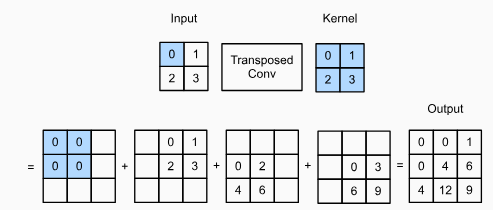
Ignoring channels for now, let’s begin with the basic transposed convolution operation with stride of 1 and no padding. Suppose that we are given a nℎ×nw input tensor and a kℎ×kw kernel. Sliding the kernel window with stride of 1 for nw times in each row and nℎ times in each column yields a total of nℎnw intermediate results. Each intermediate result is a (nℎ+kℎ−1)×(nw+kw−1) tensor that are initialized as zeros. To compute each intermediate tensor, each element in the input tensor is multiplied by the kernel so that the resulting kℎ×kw tensor replaces a portion in each intermediate tensor. Note that the position of the replaced portion in each intermediate tensor corresponds to the position of the element in the input tensor used for the computation. In the end, all the intermediate results are summed over to produce the output.
지금은 채널을 무시하고 보폭이 1이고 패딩이 없는 기본 전치 컨볼루션 작업 transposed convolution operation 부터 시작하겠습니다. nℎ×nw 입력 텐서와 kℎ×kw 커널이 주어졌다고 가정합니다. 커널 창을 각 행에서 nw번, 각 열에서 nℎ번 stride 1로 슬라이딩하면 총 nℎnw 중간 결과가 생성됩니다. 각 중간 결과는 0으로 초기화되는 (nℎ+kℎ−1)×(nw+kw−1) 텐서입니다. 각 중간 텐서를 계산하기 위해 입력 텐서의 각 요소에 커널을 곱하여 결과 kℎ×kw 텐서가 각 중간 텐서의 일부를 대체합니다. 각 중간 텐서에서 대체된 부분의 위치는 계산에 사용된 입력 텐서의 요소 위치에 해당합니다. 결국 모든 중간 결과가 합산되어 출력이 생성됩니다.
As an example, Fig. 14.10.1 illustrates how transposed convolution with a 2×2 kernel is computed for a 2×2 input tensor.
예를 들어, 그림 14.10.1은 2×2 입력 텐서에 대해 2×2 커널을 사용한 전치 컨볼루션이 계산되는 방법을 보여줍니다.
We can implement this basic transposed convolution operation trans_conv for a input matrix X and a kernel matrix K.
입력 행렬 X와 커널 행렬 K에 대해 이 기본 전치 합성곱 연산transposed convolution operation trans_conv를 구현할 수 있습니다.
def trans_conv(X, K):
    h, w = K.shape
    Y = torch.zeros((X.shape[0] + h - 1, X.shape[1] + w - 1))
    for i in range(X.shape[0]):
        for j in range(X.shape[1]):
            Y[i: i + h, j: j + w] += X[i, j] * K
    return Y
이 코드는 2D 행렬 X와 커널 행렬 K 간의 2D 전치 합성곱(Transposed Convolution) 연산을 수행하는 함수를 정의한 내용입니다.
- def trans_conv(X, K):: trans_conv 함수를 정의합니다. 이 함수는 2D 전치 합성곱 연산을 수행합니다.
- h, w = K.shape: 커널 K의 높이와 너비를 가져옵니다.
- Y = torch.zeros((X.shape[0] + h - 1, X.shape[1] + w - 1)): 출력 결과를 저장할 2D 행렬 Y를 초기화합니다. 크기는 입력 X의 높이와 너비에 커널 K의 크기를 더한 값으로 설정됩니다.
- for i in range(X.shape[0]):: 입력 X의 행 인덱스에 대해 반복합니다.
- for j in range(X.shape[1]):: 입력 X의 열 인덱스에 대해 반복합니다.
- Y[i: i + h, j: j + w] += X[i, j] * K: 입력 X의 (i, j) 위치에서 커널 K를 가중치로 사용하여 출력 Y의 해당 영역에 누적합니다.
- for j in range(X.shape[1]):: 입력 X의 열 인덱스에 대해 반복합니다.
- return Y: 전치 합성곱 연산 결과인 출력 행렬 Y를 반환합니다.
이 함수는 입력과 커널로 주어진 데이터에 대해 2D 전치 합성곱 연산을 수행하여 출력 결과를 생성합니다.
In contrast to the regular convolution (in Section 7.2) that reduces input elements via the kernel, the transposed convolution broadcasts input elements via the kernel, thereby producing an output that is larger than the input. We can construct the input tensor X and the kernel tensor K from Fig. 14.10.1 to validate the output of the above implementation of the basic two-dimensional transposed convolution operation.
커널을 통해 입력 요소를 줄이는 일반 컨볼루션(섹션 7.2)과 달리 전치 컨볼루션은 커널을 통해 입력 요소를 브로드캐스트하여 입력보다 큰 출력을 생성합니다. 그림 14.10.1에서 입력 텐서 X와 커널 텐서 K를 구성하여 기본 2차원 전치 컨볼루션 연산의 위 구현 결과를 검증할 수 있습니다.
X = torch.tensor([[0.0, 1.0], [2.0, 3.0]])
K = torch.tensor([[0.0, 1.0], [2.0, 3.0]])
trans_conv(X, K)
이 코드는 주어진 입력 행렬 X와 커널 K에 대해 2D 전치 합성곱 연산을 수행하는 과정을 나타냅니다.
- X = torch.tensor([[0.0, 1.0], [2.0, 3.0]]): 2x2 크기의 입력 행렬 X를 생성합니다.
- K = torch.tensor([[0.0, 1.0], [2.0, 3.0]]): 2x2 크기의 커널 K를 생성합니다.
- trans_conv(X, K): 앞에서 정의한 trans_conv 함수에 입력 행렬 X와 커널 K를 전달하여 전치 합성곱 연산을 수행합니다.
이 코드는 입력 행렬과 커널을 사용하여 전치 합성곱 연산을 실행한 결과를 반환합니다. 결과적으로 2D 전치 합성곱 연산의 결과를 확인할 수 있습니다.
tensor([[ 0.,  0.,  1.],
        [ 0.,  4.,  6.],
        [ 4., 12.,  9.]])
Alternatively, when the input X and kernel K are both four-dimensional tensors, we can use high-level APIs to obtain the same results.
또는 입력 X와 커널 K가 모두 4차원 텐서인 경우 고급 API를 사용하여 동일한 결과를 얻을 수 있습니다.
X, K = X.reshape(1, 1, 2, 2), K.reshape(1, 1, 2, 2)
tconv = nn.ConvTranspose2d(1, 1, kernel_size=2, bias=False)
tconv.weight.data = K
tconv(X)
이 코드는 주어진 입력 행렬 X와 커널 K에 대해 PyTorch의 합성곱 전치(Convolutional Transpose) 연산을 수행하는 과정을 나타냅니다.
- X, K = X.reshape(1, 1, 2, 2), K.reshape(1, 1, 2, 2): 입력 행렬 X와 커널 K를 4차원 텐서로 변환합니다. 이를 위해 reshape 함수를 사용하여 각각 (1, 1, 2, 2) 크기의 4차원 텐서로 변환합니다. 이는 PyTorch 합성곱 연산의 입력 형식에 맞추기 위함입니다.
- tconv = nn.ConvTranspose2d(1, 1, kernel_size=2, bias=False): PyTorch의 nn.ConvTranspose2d 클래스를 사용하여 합성곱 전치 연산을 정의합니다. 입력 채널과 출력 채널을 각각 1로 설정하고, 커널 크기를 2로 설정하며, 편향을 사용하지 않도록 bias=False로 설정합니다.
- tconv.weight.data = K: 합성곱 전치 연산의 가중치(weight)를 커널 K로 설정합니다.
- tconv(X): 정의한 합성곱 전치 연산 tconv를 입력 텐서 X에 적용하여 결과를 계산합니다. 이는 입력 X를 커널 K를 사용하여 전치 합성곱 연산을 수행한 결과입니다.
이 코드는 PyTorch의 합성곱 전치 연산을 활용하여 주어진 입력 행렬과 커널에 대한 결과를 계산하고 반환하는 과정을 나타냅니다.
tensor([[[[ 0.,  0.,  1.],
          [ 0.,  4.,  6.],
          [ 4., 12.,  9.]]]], grad_fn=<ConvolutionBackward0>)
14.10.2. Padding, Strides, and Multiple Channels
Different from in the regular convolution where padding is applied to input, it is applied to output in the transposed convolution. For example, when specifying the padding number on either side of the height and width as 1, the first and last rows and columns will be removed from the transposed convolution output.
패딩이 입력에 적용되는 일반 컨볼루션과 달리 전치 컨볼루션에서는 출력에 패딩이 적용됩니다. 예를 들어 높이와 너비 양쪽의 패딩 수를 1로 지정하면 Transposed Convolution 출력에서 첫 번째와 마지막 행과 열이 제거됩니다.
tconv = nn.ConvTranspose2d(1, 1, kernel_size=2, padding=1, bias=False)
tconv.weight.data = K
tconv(X)
이 코드는 주어진 입력 행렬 X와 커널 K에 대해 PyTorch의 패딩이 포함된 합성곱 전치(Convolutional Transpose) 연산을 수행하는 과정을 나타냅니다.
- tconv = nn.ConvTranspose2d(1, 1, kernel_size=2, padding=1, bias=False): PyTorch의 nn.ConvTranspose2d 클래스를 사용하여 패딩이 포함된 합성곱 전치 연산을 정의합니다. 입력 채널과 출력 채널을 각각 1로 설정하고, 커널 크기를 2로 설정하며, 패딩을 1로 설정하고, 편향을 사용하지 않도록 bias=False로 설정합니다. 이렇게 함으로써 입력 이미지에 패딩이 적용된 합성곱 전치 연산을 수행하게 됩니다.
- tconv.weight.data = K: 합성곱 전치 연산의 가중치(weight)를 커널 K로 설정합니다.
- tconv(X): 정의한 패딩이 포함된 합성곱 전치 연산 tconv를 입력 텐서 X에 적용하여 결과를 계산합니다. 이는 입력 X에 패딩이 적용된 상태에서 커널 K를 사용하여 전치 합성곱 연산을 수행한 결과입니다.
이 코드는 PyTorch의 패딩이 포함된 합성곱 전치 연산을 활용하여 주어진 입력 행렬과 커널에 대한 결과를 계산하고 반환하는 과정을 나타냅니다.
tensor([[[[4.]]]], grad_fn=<ConvolutionBackward0>)In the transposed convolution, strides are specified for intermediate results (thus output), not for input. Using the same input and kernel tensors from Fig. 14.10.1, changing the stride from 1 to 2 increases both the height and weight of intermediate tensors, hence the output tensor in Fig. 14.10.2.
Transposed Convolution에서 보폭은 입력이 아닌 중간 결과(따라서 출력)에 지정됩니다. 그림 14.10.1의 동일한 입력 및 커널 텐서를 사용하여 stride를 1에서 2로 변경하면 중간 텐서의 높이와 무게가 모두 증가하므로 그림 14.10.2의 출력 텐서가 증가합니다.

The following code snippet can validate the transposed convolution output for stride of 2 in Fig. 14.10.2.
다음 코드 스니펫은 그림 14.10.2에서 보폭이 2인 전치 컨볼루션 출력을 검증할 수 있습니다.
tconv = nn.ConvTranspose2d(1, 1, kernel_size=2, stride=2, bias=False)
tconv.weight.data = K
tconv(X)
이 코드는 주어진 입력 행렬 X와 커널 K에 대해 PyTorch의 스트라이드(stride)가 적용된 합성곱 전치(Convolutional Transpose) 연산을 수행하는 과정을 나타냅니다.
- tconv = nn.ConvTranspose2d(1, 1, kernel_size=2, stride=2, bias=False): PyTorch의 nn.ConvTranspose2d 클래스를 사용하여 스트라이드가 적용된 합성곱 전치 연산을 정의합니다. 입력 채널과 출력 채널을 각각 1로 설정하고, 커널 크기를 2로 설정하며, 스트라이드를 2로 설정하고, 편향을 사용하지 않도록 bias=False로 설정합니다. 이렇게 함으로써 입력 이미지에 스트라이드가 적용된 합성곱 전치 연산을 수행하게 됩니다.
- tconv.weight.data = K: 합성곱 전치 연산의 가중치(weight)를 커널 K로 설정합니다.
- tconv(X): 정의한 스트라이드가 적용된 합성곱 전치 연산 tconv를 입력 텐서 X에 적용하여 결과를 계산합니다. 이는 입력 X에 스트라이드가 적용된 상태에서 커널 K를 사용하여 전치 합성곱 연산을 수행한 결과입니다.
이 코드는 PyTorch의 스트라이드가 적용된 합성곱 전치 연산을 활용하여 주어진 입력 행렬과 커널에 대한 결과를 계산하고 반환하는 과정을 나타냅니다.
tensor([[[[0., 0., 0., 1.],
          [0., 0., 2., 3.],
          [0., 2., 0., 3.],
          [4., 6., 6., 9.]]]], grad_fn=<ConvolutionBackward0>)
For multiple input and output channels, the transposed convolution works in the same way as the regular convolution. Suppose that the input has ci channels, and that the transposed convolution assigns a kℎ×kw kernel tensor to each input channel. When multiple output channels are specified, we will have a ci×kℎ×kw kernel for each output channel.
다중 입력 및 출력 채널의 경우 전치 컨볼루션은 일반 컨볼루션과 동일한 방식으로 작동합니다. 입력에 ci 채널이 있고 전치 컨벌루션이 각 입력 채널에 kℎ×kw 커널 텐서를 할당한다고 가정합니다. 여러 출력 채널이 지정된 경우 각 출력 채널에 대해 ci×kℎ×kw 커널이 있습니다.
As in all, if we feed X into a convolutional layer f to output Y=f(X) and create a transposed convolutional layer g with the same hyperparameters as f except for the number of output channels being the number of channels in X, then g(Y) will have the same shape as X. This can be illustrated in the following example.
대체로 X를 컨볼루션 레이어 f에 공급하여 Y=f(X)를 출력하고 출력 채널 수가 X의 채널 수인 것을 제외하고 f와 동일한 하이퍼파라미터로 전치된 컨볼루션 레이어 g를 생성하면 g(Y)는 X와 동일한 모양을 갖습니다. 이는 다음 예에서 설명할 수 있습니다.
X = torch.rand(size=(1, 10, 16, 16))
conv = nn.Conv2d(10, 20, kernel_size=5, padding=2, stride=3)
tconv = nn.ConvTranspose2d(20, 10, kernel_size=5, padding=2, stride=3)
tconv(conv(X)).shape == X.shape
이 코드는 주어진 입력 텐서 X에 대해 합성곱(Convolution)과 합성곱 전치(Convolutional Transpose) 연산을 차례로 적용하고, 최종 결과의 형태를 확인하는 과정을 나타냅니다.
- X = torch.rand(size=(1, 10, 16, 16)): 크기가 (1, 10, 16, 16)인 랜덤한 값을 가지는 4차원 텐서 X를 생성합니다. 이는 1개의 채널, 10개의 필터, 16x16 크기의 이미지를 의미합니다.
- conv = nn.Conv2d(10, 20, kernel_size=5, padding=2, stride=3): 입력 채널이 10이고 출력 채널이 20인 합성곱 연산(nn.Conv2d)을 정의합니다. 커널 크기를 5로 설정하고, 패딩을 2로 설정하여 출력 크기를 입력과 같게 만들어주고, 스트라이드를 3으로 설정하여 스트라이드가 적용된 합성곱을 정의합니다.
- tconv = nn.ConvTranspose2d(20, 10, kernel_size=5, padding=2, stride=3): 입력 채널이 20이고 출력 채널이 10인 합성곱 전치 연산(nn.ConvTranspose2d)을 정의합니다. 커널 크기를 5로 설정하고, 패딩을 2로 설정하여 출력 크기를 입력과 같게 만들어주고, 스트라이드를 3으로 설정하여 스트라이드가 적용된 합성곱 전치를 정의합니다.
- tconv(conv(X)).shape == X.shape: 먼저 입력 X에 합성곱 conv를 적용한 결과에 합성곱 전치 tconv를 적용한 결과의 형태가 입력 X의 형태와 같은지 비교합니다. 이 비교 결과는 True 또는 False가 됩니다. 이 비교는 합성곱과 합성곱 전치 연산을 차례로 적용했을 때 입력과 동일한 형태의 결과가 나오는지 확인하는 것입니다.
이 코드는 PyTorch의 합성곱과 합성곱 전치 연산을 적용하고 그 결과의 형태를 확인하는 과정을 나타내며, 해당 비교를 통해 합성곱과 합성곱 전치 연산의 효과를 확인할 수 있습니다.
True
14.10.3. Connection to Matrix Transposition
The transposed convolution is named after the matrix transposition. To explain, let’s first see how to implement convolutions using matrix multiplications. In the example below, we define a 3×3 input X and a 2×2 convolution kernel K, and then use the corr2d function to compute the convolution output Y.
전치 컨볼루션은 행렬 전치의 이름을 따서 명명되었습니다. 설명을 위해 먼저 행렬 곱셈을 사용하여 컨볼루션을 구현하는 방법을 살펴보겠습니다. 아래 예에서는 3×3 입력 X와 2×2 컨볼루션 커널 K를 정의한 다음 corr2d 함수를 사용하여 컨볼루션 출력 Y를 계산합니다.
X = torch.arange(9.0).reshape(3, 3)
K = torch.tensor([[1.0, 2.0], [3.0, 4.0]])
Y = d2l.corr2d(X, K)
Y
이 코드는 주어진 입력 행렬 X와 커널 K에 대해 2D 상관(Correlation) 연산을 수행하는 과정을 나타냅니다.
- X = torch.arange(9.0).reshape(3, 3): 0부터 8까지의 값을 가지는 1차원 텐서를 3x3 크기의 2차원 행렬 X로 재구성합니다. 이는 입력 행렬입니다.
- K = torch.tensor([[1.0, 2.0], [3.0, 4.0]]): 주어진 값을 가지는 2x2 크기의 커널 행렬 K를 생성합니다. 이는 2D 상관 연산에 사용될 커널입니다.
- Y = d2l.corr2d(X, K): 2D 상관 연산 함수 d2l.corr2d를 사용하여 입력 행렬 X와 커널 K에 대해 상관 연산을 수행한 결과인 출력 행렬 Y를 계산합니다.
이 코드는 주어진 입력 행렬과 커널에 대해 2D 상관 연산을 수행하고 그 결과인 출력 행렬 Y를 반환하는 과정을 나타냅니다.
tensor([[27., 37.],
        [57., 67.]])
Next, we rewrite the convolution kernel K as a sparse weight matrix W containing a lot of zeros. The shape of the weight matrix is (4, 9), where the non-zero elements come from the convolution kernel K.
다음으로 컨볼루션 커널 K를 많은 0을 포함하는 희소 가중치 행렬 W로 다시 작성합니다. 가중치 행렬의 모양은 (4, 9)이며, 여기서 0이 아닌 요소는 컨볼루션 커널 K에서 나옵니다.
def kernel2matrix(K):
    k, W = torch.zeros(5), torch.zeros((4, 9))
    k[:2], k[3:5] = K[0, :], K[1, :]
    W[0, :5], W[1, 1:6], W[2, 3:8], W[3, 4:] = k, k, k, k
    return W

W = kernel2matrix(K)
W
이 코드는 주어진 2x2 크기의 커널 K를 행렬 형태로 변환하는 과정을 나타냅니다.
- def kernel2matrix(K): 커널 K를 입력으로 받아서 행렬 형태로 변환하는 함수 kernel2matrix를 정의합니다.
- k, W = torch.zeros(5), torch.zeros((4, 9)): 크기가 5인 1차원 텐서 k와 크기가 (4, 9)인 2차원 텐서 W를 생성합니다. k는 행렬 W를 구성하기 위한 임시 벡터입니다.
- k[:2], k[3:5] = K[0, :], K[1, :]: K의 첫 번째 행과 두 번째 행의 값을 k의 첫 번째 원소와 세 번째, 네 번째 원소에 대입합니다. 이를 통해 k 벡터에 커널 K의 값들이 할당됩니다.
- W[0, :5], W[1, 1:6], W[2, 3:8], W[3, 4:] = k, k, k, k: 행렬 W의 각 행에 k의 값들을 할당하여 행렬 형태로 변환합니다. 각 행은 서로 다른 위치에서 시작하는 값을 가지도록 할당됩니다.
- return W: 변환된 행렬 W를 반환합니다.
- W = kernel2matrix(K): 주어진 커널 K에 대해 kernel2matrix 함수를 호출하여 커널을 행렬 형태로 변환한 결과인 행렬 W를 얻습니다.
이 코드는 주어진 2x2 크기의 커널을 행렬 형태로 변환하여 행렬 W로 반환하는 과정을 나타냅니다.
tensor([[1., 2., 0., 3., 4., 0., 0., 0., 0.],
        [0., 1., 2., 0., 3., 4., 0., 0., 0.],
        [0., 0., 0., 1., 2., 0., 3., 4., 0.],
        [0., 0., 0., 0., 1., 2., 0., 3., 4.]])
Concatenate the input X row by row to get a vector of length 9. Then the matrix multiplication of W and the vectorized X gives a vector of length 4. After reshaping it, we can obtain the same result Y from the original convolution operation above: we just implemented convolutions using matrix multiplications.
입력 X를 행별로 연결하여 길이가 9인 벡터를 얻습니다. 그런 다음 W와 벡터화된 X의 행렬 곱셈은 길이가 4인 벡터를 제공합니다. 이를 재구성한 후 위의 원래 컨볼루션 연산에서 동일한 결과 Y를 얻을 수 있습니다. 방금 행렬 곱셈을 사용하여 컨볼루션을 구현했습니다.
Y == torch.matmul(W, X.reshape(-1)).reshape(2, 2)이 코드는 주어진 입력 행렬 X와 변환된 행렬 W를 사용하여 행렬-벡터 곱셈을 수행한 결과인 출력 행렬 Y가 정확히 일치하는지를 확인하는 조건을 나타냅니다.
- Y: 위 코드에서 계산한 행렬 Y입니다.
- torch.matmul(W, X.reshape(-1)): 행렬 W와 입력 행렬 X를 벡터로 펼친 뒤, 행렬-벡터 곱셈을 수행한 결과입니다.
- .reshape(2, 2): 이전 계산 결과를 2x2 크기의 행렬로 재구성합니다.
- ==: 두 행렬이 원소별로 일치하는지를 비교하는 연산자입니다.
따라서, 위 코드는 변환된 행렬 W와 입력 행렬 X를 사용하여 계산한 출력 행렬 Y가 정확히 일치하는지 여부를 확인하고 그 결과를 반환하는 조건을 나타냅니다.
tensor([[True, True],
        [True, True]])
Likewise, we can implement transposed convolutions using matrix multiplications. In the following example, we take the 2×2 output Y from the above regular convolution as input to the transposed convolution. To implement this operation by multiplying matrices, we only need to transpose the weight matrix W with the new shape (9,4).
마찬가지로 행렬 곱셈을 사용하여 전치 컨볼루션을 구현할 수 있습니다. 다음 예제에서는 위의 일반 컨볼루션에서 2×2 출력 Y를 전치 컨볼루션의 입력으로 사용합니다. 행렬을 곱하여 이 연산을 구현하려면 가중치 행렬 W를 새 모양(9,4)으로 바꾸면 됩니다.
Z = trans_conv(Y, K)
Z == torch.matmul(W.T, Y.reshape(-1)).reshape(3, 3)
이 코드는 주어진 출력 행렬 Y와 변환된 행렬 W를 사용하여 역변환 행렬-벡터 곱셈을 수행한 결과인 행렬 Z가 정확히 일치하는지를 확인하는 조건을 나타냅니다.
- Z: trans_conv 함수를 사용하여 계산한 행렬 Z입니다.
- trans_conv(Y, K): 출력 행렬 Y와 주어진 커널 K를 사용하여 역변환 행렬-벡터 곱셈을 수행한 결과입니다.
- torch.matmul(W.T, Y.reshape(-1)): 행렬 W의 전치 행렬과 Y를 벡터로 펼친 뒤, 역변환 행렬-벡터 곱셈을 수행한 결과입니다.
- .reshape(3, 3): 이전 계산 결과를 3x3 크기의 행렬로 재구성합니다.
- ==: 두 행렬이 원소별로 일치하는지를 비교하는 연산자입니다.
따라서, 위 코드는 주어진 출력 행렬 Y와 변환된 행렬 W를 사용하여 역변환 행렬-벡터 곱셈을 수행한 결과인 행렬 Z가 정확히 일치하는지 여부를 확인하고 그 결과를 반환하는 조건을 나타냅니다.
tensor([[True, True, True],
        [True, True, True],
        [True, True, True]])
Consider implementing the convolution by multiplying matrices. Given an input vector x and a weight matrix W, the forward propagation function of the convolution can be implemented by multiplying its input with the weight matrix and outputting a vector y=Wx. Since backpropagation follows the chain rule and ∇xy=W⊤, the backpropagation function of the convolution can be implemented by multiplying its input with the transposed weight matrix W⊤. Therefore, the transposed convolutional layer can just exchange the forward propagation function and the backpropagation function of the convolutional layer: its forward propagation and backpropagation functions multiply their input vector with W⊤ and W, respectively.
행렬을 곱하여 컨벌루션을 구현하는 것을 고려하십시오. 입력 벡터 x와 가중치 행렬 W가 주어지면 컨볼루션의 순방향 전파 함수는 입력에 가중치 행렬을 곱하고 벡터 y=Wx를 출력하여 구현할 수 있습니다. 역전파는 체인 규칙과 ∇xy=W⊤를 따르기 때문에 컨볼루션의 역전파 함수는 전치된 가중치 행렬 W⊤를 입력에 곱하여 구현할 수 있습니다. 따라서 전치된 컨볼루션 레이어는 컨볼루션 레이어의 순방향 전파 함수와 역전파 함수를 교환할 수 있습니다. 순방향 전파 및 역전파 함수는 각각 입력 벡터에 W⊤ 및 W를 곱합니다.
14.10.4. Summary
- In contrast to the regular convolution that reduces input elements via the kernel, the transposed convolution broadcasts input elements via the kernel, thereby producing an output that is larger than the input.
커널을 통해 입력 요소를 줄이는 일반 컨볼루션과 달리 전치 컨볼루션은 커널을 통해 입력 요소를 브로드캐스팅하여 입력보다 큰 출력을 생성합니다. - If we feed X into a convolutional layer f to output Y=f(X) and create a transposed convolutional layer g with the same hyperparameters as f except for the number of output channels being the number of channels in X, then g(Y) will have the same shape as X.
X를 컨볼루션 레이어 f에 공급하여 Y=f(X)를 출력하고 출력 채널 수가 X의 채널 수인 것을 제외하고 f와 동일한 하이퍼파라미터로 전치된 컨볼루션 레이어 g를 생성하면 g(Y) X와 같은 모양을 갖게 됩니다. - We can implement convolutions using matrix multiplications. The transposed convolutional layer can just exchange the forward propagation function and the backpropagation function of the convolutional layer.
행렬 곱셈을 사용하여 컨볼루션을 구현할 수 있습니다. Transposed convolutional layer는 convolutional layer의 forward propagation function과 backpropagation function을 교환할 수 있습니다.
14.10.5. Exercises
- In Section 14.10.3, the convolution input X and the transposed convolution output Z have the same shape. Do they have the same value? Why?
- Is it efficient to use matrix multiplications to implement convolutions? Why?
'Dive into Deep Learning > D2L Computer Vision' 카테고리의 다른 글
| D2L - 14.12. Neural Style Transfer (1) | 2023.08.21 |
|---|---|
| D2L - 14.11. Fully Convolutional Networks (0) | 2023.08.21 |
| D2L - 14.9. Semantic Segmentation and the Dataset (0) | 2023.08.20 |
| D2L - 14.8. Region-based CNNs (R-CNNs) (0) | 2023.08.20 |
| D2L - 14.7. Single Shot Multibox Detection (0) | 2023.08.19 |
| D2L - 14.6. The Object Detection Dataset (0) | 2023.08.19 |
| D2L - 14.5. Multiscale Object Detection (0) | 2023.08.19 |
| D2L - 14.4. Anchor Boxes (0) | 2023.08.19 |
| D2L - 14.3. Object Detection and Bounding Boxes (0) | 2023.08.19 |
| D2L - 14.2. Fine-Tuning (0) | 2023.08.19 |