개발자로서 현장에서 일하면서 새로 접하는 기술들이나 알게된 정보 등을 정리하기 위한 블로그입니다. 운 좋게 미국에서 큰 회사들의 프로젝트에서 컬설턴트로 일하고 있어서 새로운 기술들을 접할 기회가 많이 있습니다. 미국의 IT 프로젝트에서 사용되는 툴들에 대해 많은 분들과 정보를 공유하고 싶습니다.
In this example we'll try to go over all operations that can be done using the Azure endpoints and their differences with the openAI endpoints (if any).
이 예제에서는 Azure endpoints 를 사용하여 수행할 수 있는 모든 작업과 openAI endpoints(있는 경우)과의 차이점을 살펴보겠습니다.
This example focuses on finetuning but also touches on the majority of operations that are available using the API. This example is meant to be a quick way of showing simple operations and is not meant as a finetune model adaptation tutorial.
이 예제는 finetuning에 중점을 두지만 API를 사용하여 사용할 수 있는 대부분의 작업도 다룹니다. 이 예제는 간단한 작업을 빠르게 보여주기 위한 것이며 finetuning 모델 적용 튜토리얼이 아닙니다.
import openai
from openai import cli
Setup
For the following sections to work properly we first have to setup some things. Let's start with theapi_baseandapi_version. To find yourapi_basego tohttps://portal.azure.com, find your resource and then under "Resource Management" -> "Keys and Endpoints" look for the "Endpoint" value.
다음 섹션이 제대로 작동하려면 먼저 몇 가지를 설정해야 합니다. api_base 및 api_version부터 시작하겠습니다. api_base를 찾으려면 https://portal.azure.com으로 이동하여 리소스를 찾은 다음 "Resource Management" -> "Keys and Endpoints"에서 "Endpoint" 값을 찾습니다.
openai.api_version = '2022-12-01'
openai.api_base = '' # Please add your endpoint here
We next have to setup theapi_typeandapi_key. We can either get the key from the portal or we can get it through Microsoft Active Directory Authentication. Depending on this theapi_typeis eitherazureorazure_ad.
다음으로 api_type 및 api_key를 설정해야 합니다. 포털에서 키를 얻거나 Microsoft Active Directory 인증을 통해 얻을 수 있습니다. 이에 따라 api_type은 azure 또는 azure_ad입니다.
Setup: Portal
Let's first look at getting the key from the portal. Go tohttps://portal.azure.com, find your resource and then under "Resource Management" -> "Keys and Endpoints" look for one of the "Keys" values.
먼저 포털에서 키를 가져오는 방법을 살펴보겠습니다. https://portal.azure.com으로 이동하여 리소스를 찾은 다음 "Resource Management" -> "Keys and Endpoints"에서 "Keys" 값 중 하나를 찾습니다.
openai.api_type = 'azure'
openai.api_key = ''  # Please add your api key here
(Optional) Setup: Microsoft Active Directory Authentication
Let's now see how we can get a key via Microsoft Active Directory Authentication. Uncomment the following code if you want to use Active Directory Authentication instead of keys from the portal.
(선택 사항) 설정: Microsoft Active Directory 인증 이제 Microsoft Active Directory 인증을 통해 키를 얻는 방법을 살펴보겠습니다. 포털의 키 대신 Active Directory 인증을 사용하려면 다음 코드의 주석을 제거하십시오.
In the next section we will focus on the files operations: importing, listing, retrieving, deleting. For this we need to create 2 temporary files with some sample data. For the sake of simplicity, we will use the same data for training and validation.
다음 섹션에서는 가져오기, 나열, 검색, 삭제와 같은 파일 작업에 중점을 둘 것입니다. 이를 위해 일부 샘플 데이터로 2개의 임시 파일을 생성해야 합니다. 단순화를 위해 교육 및 검증에 동일한 데이터를 사용합니다.
import shutil
import json

training_file_name = 'training.jsonl'
validation_file_name = 'validation.jsonl'

sample_data = [{"prompt": "When I go to the store, I want an", "completion": "apple."},
    {"prompt": "When I go to work, I want a", "completion": "coffee."},
    {"prompt": "When I go home, I want a", "completion": "soda."}]

print(f'Generating the training file: {training_file_name}')
with open(training_file_name, 'w') as training_file:
    for entry in sample_data:
        json.dump(entry, training_file)
        training_file.write('\n')

print(f'Copying the training file to the validation file')
shutil.copy(training_file_name, validation_file_name)
Files: Listing
List all of the uploaded files and check for the ones that are named "training.jsonl" or "validation.jsonl"
업로드된 모든 파일을 나열하고 이름이 "training.jsonl" 또는 "validation.jsonl"인 파일을 확인합니다.
print('Checking for existing uploaded files.')
results = []
files = openai.File.list().data
print(f'Found {len(files)} total uploaded files in the subscription.')
for item in files:
    if item["filename"] in [training_file_name, validation_file_name]:
        results.append(item["id"])
print(f'Found {len(results)} already uploaded files that match our names.')
Files: Deleting
Let's now delete those found files (if any) since we're going to be re-uploading them next.
다음에 다시 업로드할 예정이므로 찾은 파일(있는 경우)을 삭제하겠습니다.
print(f'Deleting already uploaded files...')
for id in results:
    openai.File.delete(sid = id)
Files: Importing & Retrieving
Now, let's import our two files ('training.jsonl' and 'validation.jsonl') and keep those IDs since we're going to use them later for finetuning.
이제 두 파일('training.jsonl' 및 'validation.jsonl')을 가져오고 나중에 미세 조정에 사용할 것이므로 해당 ID를 유지하겠습니다.
For this operation we are going to use the cli wrapper which does a bit more checks before uploading and also gives us progress. In addition, after uploading we're going to check the status our import until it has succeeded (or failed if something goes wrong)
이 작업을 위해 업로드하기 전에 조금 더 확인하고 진행률을 제공하는 cli 래퍼를 사용할 것입니다. 또한 업로드 후 가져오기가 성공할 때까지(또는 무언가 잘못되면 실패할 때까지) 가져오기 상태를 확인합니다.
import time

def check_status(training_id, validation_id):
    train_status = openai.File.retrieve(training_id)["status"]
    valid_status = openai.File.retrieve(validation_id)["status"]
    print(f'Status (training_file | validation_file): {train_status} | {valid_status}')
    return (train_status, valid_status)

#importing our two files
training_id = cli.FineTune._get_or_upload(training_file_name, True)
validation_id = cli.FineTune._get_or_upload(validation_file_name, True)

#checking the status of the imports
(train_status, valid_status) = check_status(training_id, validation_id)

while train_status not in ["succeeded", "failed"] or valid_status not in ["succeeded", "failed"]:
    time.sleep(1)
    (train_status, valid_status) = check_status(training_id, validation_id)
Files: Downloading
Now let's download one of the files, the training file for example, to check that everything was in order during importing and all bits are there.
이제 파일 중 하나(예: 교육 파일)를 다운로드하여 가져오는 동안 모든 것이 제대로 작동하고 모든 비트가 있는지 확인합니다.
print(f'Downloading training file: {training_id}')
result = openai.File.download(training_id)
print(result.decode('utf-8'))
Finetune
In this section we are going to use the two training and validation files that we imported in the previous section, to train a finetune model.
이 섹션에서는 finetune 모델을 교육하기 위해 이전 섹션에서 가져온 두 개의 교육 및 검증 파일을 사용할 것입니다.
While the job runs, we can subscribe to the streaming events to check the progress of the operation.
작업이 실행되는 동안 스트리밍 이벤트를 구독하여 작업 진행 상황을 확인할 수 있습니다.
import signal
import datetime

def signal_handler(sig, frame):
    status = openai.FineTune.retrieve(job_id).status
    print(f"Stream interrupted. Job is still {status}.")
    return

print(f'Streaming events for the fine-tuning job: {job_id}')
signal.signal(signal.SIGINT, signal_handler)

events = openai.FineTune.stream_events(job_id)
try:
    for event in events:
        print(f'{datetime.datetime.fromtimestamp(event["created_at"])} {event["message"]}')

except Exception:
    print("Stream interrupted (client disconnected).")
Finetune: Listing and Retrieving
Now let's check that our operation was successful and in addition we can look at all of the finetuning operations using a list operation.
이제 작업이 성공했는지 확인하고 목록 작업을 사용하여 모든 finetune 작업을 볼 수 있습니다.
status = openai.FineTune.retrieve(id=job_id)["status"]
if status not in ["succeeded", "failed"]:
    print(f'Job not in terminal status: {status}. Waiting.')
    while status not in ["succeeded", "failed"]:
        time.sleep(2)
        status = openai.FineTune.retrieve(id=job_id)["status"]
        print(f'Status: {status}')
else:
    print(f'Finetune job {job_id} finished with status: {status}')

print('Checking other finetune jobs in the subscription.')
result = openai.FineTune.list()
print(f'Found {len(result.data)} finetune jobs.')
Finetune: Deleting
Finally we can delete our finetune job. WARNING: Please skip this step if you want to continue with the next section as the finetune model is needed. (The delete code is commented out by default)
마지막으로 finetune 작업을 삭제할 수 있습니다. 경고: finetune모델이 필요하므로 다음 섹션을 계속하려면 이 단계를 건너뛰십시오. (삭제 코드는 기본적으로 주석 처리됨)
# openai.FineTune.delete(sid=job_id)
Deployments
In this section we are going to create a deployment using the finetune model that we just adapted and then used the deployment to create a simple completion operation.
이 섹션에서는 방금 수정한 finetune 모델을 사용하여 deployment를 생성한 다음 deployment를 사용하여 간단한 completion 작업을 생성할 것입니다.
Deployments: Create
Let's create a deployment using the fine-tune model.
fine-tune모델을 사용하여 deployment를 생성해 보겠습니다.
#Fist let's get the model of the previous job:
result = openai.FineTune.retrieve(id=job_id)
if result["status"] == 'succeeded':
    model = result["fine_tuned_model"]

# Now let's create the deployment
print(f'Creating a new deployment with model: {model}')
result = openai.Deployment.create(model=model, scale_settings={"scale_type":"standard"})
deployment_id = result["id"]
Deployments: Retrieving
Now let's check the status of the newly created deployment
이제 새로 생성된 배포의 상태를 확인하겠습니다.
print(f'Checking for deployment status.')
resp = openai.Deployment.retrieve(id=deployment_id)
status = resp["status"]
print(f'Deployment {deployment_id} is with status: {status}')
Deployments: Listing
Now because creating a new deployment takes a long time, let's look in the subscription for an already finished deployment that succeeded.
이제 새 deployment를 만드는 데 시간이 오래 걸리므로 이미 완료된 deployment에 대한 subscription을 살펴보겠습니다.
print('While deployment running, selecting a completed one.')
deployment_id = None
result = openai.Deployment.list()
for deployment in result.data:
    if deployment["status"] == "succeeded":
        deployment_id = deployment["id"]
        break

if not deployment_id:
    print('No deployment with status: succeeded found.')
else:
    print(f'Found a successful deployment with id: {deployment_id}.')
Completions
Now let's send a sample completion to the deployment.
이제 deployment에 샘플 completion 을 보내겠습니다.
print('Sending a test completion job')
start_phrase = 'When I go home, I want a'
response = openai.Completion.create(deployment_id=deployment_id, prompt=start_phrase, temperature=0, stop=".")
text = response['choices'][0]['text'].replace('\n', '').replace(' .', '.').strip()
print(f'"{start_phrase} {text}."')
아래 예제는 ada 모델을 이용해서 이메일 내용을 보고 이게 Baseball과 연관 돼 있는지 아니면 Hockey와 연관 돼 있는 건지 GPT-3 가 인지할 수 있도록 Fine-Tuning을 사용해서 훈련시키고 새로운 모델을 만드는 과정을 보여 줍니다.
from sklearn.datasets import fetch_20newsgroups
import pandas as pd
import openai

categories = ['rec.sport.baseball', 'rec.sport.hockey']
sports_dataset = fetch_20newsgroups(subset='train', shuffle=True, random_state=42, categories=categories)
이 예제에서 사용하는 데이터는 sklearn에서 제공하는 샘플 데이터인 fetch_20newsgroups를 사용합니다.
fetch_20newsgroups 는 데이터를 다루는 연습용으로 만들어진 데이터 세트 입니다.
20개의 newsgroup에서 데이터를 가져온 겁니다. 이 뉴스그룹들은 대부분 게시판이고 사용자들이 올른 글들이 데이터가 되는 겁니다. 예를 들어 내가 낚시에 관심이 있어서 낚시 관련된 카페 같은 뉴스 그룹에 가입하고 거기에 글을 올리듯이 사람들이 글을 올린 데이터 들 입니다.
여기에는 20개의 주제들이 있습니다. 그리고 총 샘플들은 18846개가 있고 1차원 배열이고 text로 이뤄져 있습니다.
이 중에서 Baseball 과 Hockey 관련된 데이터를 가지고 이 예제에서는 Fine-Tuning을 연습하는 소스코드를 만들게 됩니다.
관련 모듈을 import 한 다음에 한 일은 이 예제에서 다룰 topic들을 선택하는 겁니다. 이 두 topic들을 categories라는 배열 변수에 아이템으로 넣습니다.
그리고 sports_dataset 라는 변수에 이 fetch_20newsgroups에 있는 데이터 들 중 위에서 선택한 rec.sport.baseball과 rec.sport.hockey 뉴스그룹에 있는 데이터들만 담습니다.
데이터를 다루려면 우선 그 데이터으 구조를 잘 알아야 합니다.
이 데이터의 첫번째 데이터만 한번 출력해 보겠습니다.
print(sports_dataset['data'][0])
그러면 결과는 이렇게 나옵니다.
From: dougb@comm.mot.com (Doug Bank)
Subject: Re: Info needed for Cleveland tickets
Reply-To: dougb@ecs.comm.mot.com
Organization: Motorola Land Mobile Products Sector
Distribution: usa
Nntp-Posting-Host: 145.1.146.35
Lines: 17

In article <1993Apr1.234031.4950@leland.Stanford.EDU>, bohnert@leland.Stanford.EDU (matthew bohnert) writes:

|> I'm going to be in Cleveland Thursday, April 15 to Sunday, April 18.
|> Does anybody know if the Tribe will be in town on those dates, and
|> if so, who're they playing and if tickets are available?

The tribe will be in town from April 16 to the 19th.
There are ALWAYS tickets available! (Though they are playing Toronto,
and many Toronto fans make the trip to Cleveland as it is easier to
get tickets in Cleveland than in Toronto.  Either way, I seriously
doubt they will sell out until the end of the season.)

--
Doug Bank                       Private Systems Division
dougb@ecs.comm.mot.com          Motorola Communications Sector
dougb@nwu.edu                   Schaumburg, Illinois
dougb@casbah.acns.nwu.edu       708-576-8207
데이터는 글을 올린사람, 주제, Reply-To,, Organization, Distribution, 아이피 주소. 라인 수, 내용 등등등 ...
대충 어떤 식으로 데이터들이 구성 돼 있는지 알 수 있을 것 같습니다.
이건 sports_dataset 의 data라는 아이템에 들어 있는 첫 번째 데이터인 것이고 이 sports_dataset은 어떤 구조로 돼 있는지 한번 알아 볼까요?
결과의 일 부분인데요. sports_dataset 배열은 첫번째 item 이 data 입니다. 그리고 이 data 안에는 여러 글들이 있습니다. 각 글들은 From: 으로 시작합니다. 첫번째 글은 바로 위에서 출력한 그 글입니다. dougb@comm.mot.com으로 시작해서 708-576-8207 로 끝납니다.
data는 이렇게 구성이 돼 있고 그렇다면 다른 아이템에는 무엇이 있을 까요?
그 다음에는 target_names인데 이 변수에는 baseball과 hockey 토픽만 들어 있다는걸 확인 할 수 있습니다.
그리고 'target' : array(0,1,0...,... 이렇게 돼 있는 것은 data의 첫번째 데이터는 baseball 뉴스그룹에서 온 것이고 두번째 데이터는 hockey 그룹에서 그리고 세번째는 baseball 그룹에서 온 것이라는 것을 말합니다.
data에 있는 데이터 가지고는 이것이 어느 뉴스그룹 소속인지 알 수 없는데 이 target_names 라는 두번째 아이템에서 그 정보를 얻을 수 있네요.
오늘 다룰 Fine-Tunning 예제에서는 이 두가지 정보만 있으면 GPT-3 AI 를 훈련 시킬 수 있습니다.
len_all, len_baseball, len_hockey = len(sports_dataset.data), len([e for e in sports_dataset.target if e == 0]), len([e for e in sports_dataset.target if e == 1])
print(f"Total examples: {len_all}, Baseball examples: {len_baseball}, Hockey examples: {len_hockey}")
len(sports_dataset.data) 는 이 sports_dataset에 있는 data 아이템에 있는 데이터 수를 가져 옵니다.
len([e for e in sports_dataset.target if e == 0] 는 data에 있는 데이터 중 target 이 0인 데이터 즉 rec.sport.baseball에 속한 데이터만 가져 옵니다.
같은 방법으로 Hockey 에 속한 데이터만 가져 오려면 이러헥 사용 합니다. len([e for e in sports_dataset.target if e == 1]
결과는 아래와 같습니다.
Total examples: 1197, Baseball examples: 597, Hockey examples: 600
전체 데이터 갯수는 1197개이고 야구와 관련된 글은 597개 그리고 하키와 관련된 글은 600개 입니다.
이제 이 데이터의 구조에 대해서 어느정도 파악을 했습니다.
그러면 이 데이터를 Fune-Tuning 시키기 위한 구조로 바꾸어 주어야 합니다.
Fine-Tunning은 AI를 교육 시키는 겁니다. 이 AI를 교육시키기 위해서는 데이터를 제공해야 합니다.
GPT-3라는 AI가 알아 들을 수 있는 데이터 구조는 이전 Guide에서 설명 된 부분이 있습니다.
GPT-3는 Prompt 와 Completion 이 두 부분으로 나뉘어진 데이터세트를 제공하면 됩니다.
그러면 이 아이는 그것을 보고 패턴을 찾아내서 학습하게 되는 겁니다.
이런 내용의 글은 야구와 관련 돼 있고 또 저런 내용의 글은 하키와 관련 돼 있다는 것을 알아 내는 것이죠.
예를 들어 위에서 출력한 첫번째 글을 보시죠.
여기에는 이 글이 야구와 관련돼 있는지 하키와 관련 돼 있는지에 대한 명시적인 정보는 없습니다.
다면 이 글에는 Cleveland에 갈거고 팬들끼리 좀 모이자는 내용이 있습니다. 그리고 상대팀 이름도 있고 어디서 경기가 열리는지 뭐 이런 정보가 있습니다.
미국에서 야구에 대해 관심 있는 사람이라면 이 글은 야구와 관련된 글이라는 것을 알겠죠.
이렇게 주어진 정보만 가지고 이게 야구와 관련된 글인지 하키와 관련된 글인지 알아 내도록 GPT-3를 훈련 시킬 겁니다.
그 훈련된 AI모델은 나만의 모델이 될 겁니다.
그래서 앞으로 내가 어떤 글을 그 모델에게 보내면 그 Custom AI Model은 그게 야구와 관련된 글인지 하키와 관련된 글인지를 저에게 알려 줄 것입니다.
그러면 GPT-3를 훈련 시키기 위한 데이터 세트 형식으로 위 데이터를 변경 시켜 보겠습니다.
Prompt 와 Completion 이 두가지 컬럼이 있어야 합니다.
Prompt에는 data 정보들이 있고 Completion에는 그 글이 야구와 관련된 글인지 하키와 관련된 글인지에 대한 정보들이 들거 갈 겁니다.
import pandas as pd
labels = [sports_dataset.target_names[x].split('.')[-1] for x in sports_dataset['target']]
texts = [text.strip() for text in sports_dataset['data']]
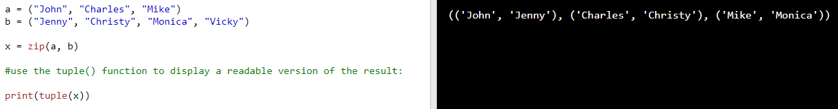
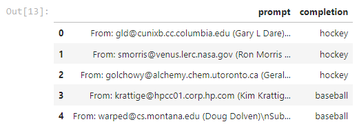
df = pd.DataFrame(zip(texts, labels), columns = ['prompt','completion']) #[:300]
df.head()
파이썬에서 데이터를 다루는 모델은 pandas를 많이 사용 합니다.
labels 부분을 보겠습니다.
위에서 sports_dataset['target'] 에는 0 과 1이라는 정보들이 있고 이 정보는 data에 있는 정보가 targetnames 의 첫번째 인수에 속하는 건지 두번째 인수에 속하는 건지를 알려 주는 것이라고 했습니다.
첫번째 인수는 rec.sport.baseball이고 두번째 인수는 rec.sport.hockey 입니다.
이 target 값에 대한 for 문이 도는데요 data 갯수가 1197이고 target의 각 인수들 (0,1) 은 각 데이터의 인수들과 매핑 돼 있으니까 이 for 문은 1197번 돌 겁니다. 이렇게 돌면서 target_names에서 해당 인수를 가져 와서 . 으로 그 텍스트를 분리 한 다음에 -1 번째 즉 맨 마지막 글자를 가지고 오게 됩니다. 그러면 baseball과 hockey라는 글자만 선택 되게 되죠.
즉 labels에는 baseball 과 hockey라는 글자들이 들어가게 되는데 이는 target 에 0이 있으면 baseball 1이 있으면 hockey가 들어가는 1197개의 인수를 가지고 있는 배열이 순서대로 들어가게 되는 겁니다.
그러면 이제 data에 있는 각 데이터를 순서대로 배열로 집어 넣으면 되겠죠?
texts = [text.strip() for text in sports_dataset['data']]
이 부분이 그 일을 합니다.
sports_dataset 에 있는 data 만큼 for 문을 돕니다. data는 1197개의 인수를 가지고 있으니 이 for 문도 1197번 돌 겁니다.
이 데이터를 그냥 texts 라는 변수에 배열 형태로 집어 넣는 겁니다. text.strip()은 해당 text의 앞 뒤에 있는 공백들을 제거 하는 겁니다.
이 부분도 중요 합니다. 데이터의 앞 뒤 공백을 제거해서 깨끗한 데이터를 만듭니다.
이제 data의 각 글을 가지고 있는 배열과 각 글들이 어느 주제에 속하는지에 대한 정보를 가지고 있는 배열들이 완성 됐습니다.
이 정보를 가지고 pandas로 GPT-3 AI 를 훈련 시킬 수 있는 형태의 데이터 세트로 만들겠습니다.
zip(texts, labels) <- 이렇게 하면 데이터와 topic이 짝 지어 지겠죠.
이 값은 pandas의 DataFrame의 첫번째 인수로 전달 되고 두번째 인수로는 컬럼 이름이 전달 됩니다. (columns = ['prompt','completion'])
그 다음 df.head() 로 이렇게 만들어진 DataFrame에서 처음에 오는 5개의 데이터를 출력해 봅니다.
의도한 대로 각 게시글과 그 게시글이 baseball에 속한 것인지 hockey에 속한 것인지에 대한 정보가 있네요.
이 cookbook에는 300개의 데이터만 사용할 것이라고 돼 있는데 어디에서 그게 돼 있는지 모르겠네요.
len() 을 찍어봐도 1197 개가 찍힙니다.
cookbook 설명대로 300개의 데이터만 사용하려면 아래와 같이 해야 할 것 같습니다.
import pandas as pd

labels = [sports_dataset.target_names[x].split('.')[-1] for x in sports_dataset['target']]
texts = [text.strip() for text in sports_dataset['data']]
df = pd.DataFrame(zip(texts, labels), columns = ['prompt','completion']) #[:300]
df = df.head(300)
print(df)
저는 이 300개의 데이터만 이용하겠습니다.
GPT-3 의 Fine-tuning 을 사용할 때 데이터 크기에 따라서 과금 될 거니까.. 그냥 조금만 하겠습니다. 지금은 공부하는 단계이니까 Custom model의 정확도 보다는 Custom model을 Fine tuning을 사용해서 만드는 과정을 배우면 되니까요.
openai aools fine_tunes.prepare_data는 데이터를 검증하고 제안하고 형식을 다시 지정해 주는 툴입니다.
위 결과를 보면 Analyzing... (분석중)으로 시작해서 이 파일에는 총 300개의 prompt-completion 쌍이 있고 모델을 fine-tune 하려고 하는 것 같은데 저렴한 ada 모델을 사용하세요... 뭐 이렇게 분석과 제안내용이 표시됩니다.
그리고 너무 긴 글이 3개 있고 134, 200,281 번째 줄. .....이렇게 나오고 이 3개는 너무 길어서 제외한다고 나오네요.
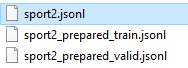
이 결과로 sport2_prepared_train.jsonl 과 sport2_prepared_valid.jsonl 파일 두개를 만들어 냅니다.
그리고 이제 fine_tunes.create을 사용해서 fine-tuning을 하면 된다고 나오네요.
Fine-tuning을 하게 되면 curie 모델을 사용하면 대략 9분 46초 정도 걸릴 것이고 ada 모델을 사용하면 그보다 더 조금 걸릴 거라네요.
폴더를 다시 봤더니 정말 두개의 jsonl 파일이 더 생성 되었습니다.
sport2_prepared_train.jsonl에는 위에 너무 길다는 3개의 데이터를 없앤 나머지 297개의 데이터가 있습니다.
sport2_prepared_valid.jsonl에는 60개의 데이터가 있습니다.
train 데이터와 valid 데이터 이렇게 두개가 생성 되었네요. 이 두개를 생성한 이유는 나중에 새 데이터에 대한 예상 성능을 쉽게 측정하기 위해서 GPT-3 의 fine_tunes.prepare_data 함수가 만든 겁니다.
Fine-tuning
이제 다 준비가 됐습니다. 실제로 Fine tuning을 하면 됩니다.
참고로 지금 우리는 내용을 주면 이 내용이 야구에 대한건지 하키에 대한건지 분류 해 주는 fine tuned 된 모델을 생성하려고 합니다.
이 작업은 classification task에 속합니다.
그래서 train 과 valid 두 데이터 세트가 위에서 생성된 거구요.
이제 Fine-tuning을 하기 위해 아래 명령어를 사용하면 됩니다.
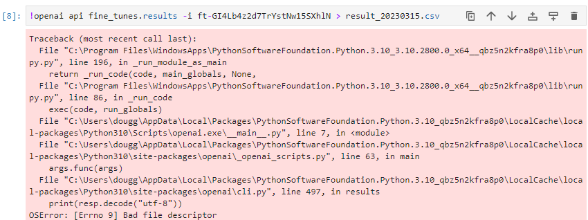
!openai api fine_tunes.create -t "sport2_prepared_train.jsonl" -v "sport2_prepared_valid.jsonl" --compute_classification_metrics --classification_positive_class " baseball" -m ada
fine_tunes.create 함수를 사용했고 training data로는 sport2_prepared_train.jsonl 파일이 있고 valid data로는 sport2.prepared_valid_jsonl이 제공된다고 돼 있습니다.
그 다음엔 compute_classification_metrics와 classification_positive_class "baseball" 이 주어 졌는데 이는 위에서 fine_tunes.prepare_data 에서 추천한 내용입니다. classification metics를 계산하기 위해 필요하기 때문에 추천 했습니다.
그리고 마지막에 -m ada는 ada 모델을 사용하겠다는 겁니다.
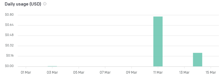
이 부분을 실행하면 요금이 청구가 됩니다.
Fine-tuning models 같은 경우 과금은 아래와 같이 됩니다.
ada 모델을 사용하니까 토큰 1천개당 0.0004불이 training 과정에 들게 됩니다.
Usage도 있네요 나중에 Fine Tune 된 Custom Model을 사용하게 되면 토큰 1천개당 0.0016 불이 과금 됩니다.
test = pd.read_json('sport2_prepared_valid.jsonl', lines=True)
test.head()
We need to use the same separator following the prompt which we used during fine-tuning. In this case it is\n\n###\n\n. Since we're concerned with classification, we want the temperature to be as low as possible, and we only require one token completion to determine the prediction of the model.
fine-tuning 중에 사용한 프롬프트 다음에 동일한 구분 기호를 사용해야 합니다. 이 경우 \n\n###\n\n입니다. 우리는 분류와 관련이 있기 때문에 temperature가 가능한 한 낮아지기를 원하며 모델의 예측을 결정하기 위해 하나의 token completion만 필요합니다.
We can see that the model predicts hockey as a lot more likely than baseball, which is the correct prediction. By requesting log_probs, we can see the prediction (log) probability for each class.
모델이 야구보다 하키를 훨씬 더 많이 예측한다는 것을 알 수 있습니다. 이것이 정확한 예측입니다. log_probs를 요청하면 각 클래스에 대한 예측(로그) 확률을 볼 수 있습니다.
Generalization
Interestingly, our fine-tuned classifier is quite versatile. Despite being trained on emails to different mailing lists, it also successfully predicts tweets.
흥미롭게도 fine-tuned classifier는 매우 다재다능합니다. 다른 메일링 리스트에 대한 이메일에 대한 교육을 받았음에도 불구하고 트윗을 성공적으로 예측합니다.
sample_hockey_tweet = """Thank you to the
@Canes
 and all you amazing Caniacs that have been so supportive! You guys are some of the best fans in the NHL without a doubt! Really excited to start this new chapter in my career with the
@DetroitRedWings
 !!"""
res = openai.Completion.create(model=ft_model, prompt=sample_hockey_tweet + '\n\n###\n\n', max_tokens=1, temperature=0, logprobs=2)
res['choices'][0]['text']
이 내용은 이전에 없던 내용 입니다..
내용에 NHL이라는 단어가 있네요. National Hockey league 겠죠?
그러면 이 이메일은 하키와 관련한 이메일 일 겁니다.
Fine tuning으로 만든 새로운 모델도 이것을 정확하게 맞춥니다.
' hockey'
sample_baseball_tweet="""BREAKING: The Tampa Bay Rays are finalizing a deal to acquire slugger Nelson Cruz from the Minnesota Twins, sources tell ESPN."""
res = openai.Completion.create(model=ft_model, prompt=sample_baseball_tweet + '\n\n###\n\n', max_tokens=1, temperature=0, logprobs=2)
res['choices'][0]['text']
그 다음 예제에서는 Tampa Bay Rays , Minnesota Twins 라는 내용이 나옵니다.
This document is a draft of a guide that will be added to the next revision of the OpenAI documentation. If you have any feedback, feel free to let us know.
이 문서는 OpenAI 문서의 다음 개정판에 추가될 가이드의 초안입니다. 의견이 있으시면 언제든지 알려주십시오.
One note: this doc shares metrics for text-davinci-002, but that model is not yet available for fine-tuning.
참고: 이 문서는 text-davinci-002에 대한 메트릭을 공유하지만 해당 모델은 아직 미세 조정에 사용할 수 없습니다.
Best practices for fine-tuning GPT-3 to classify text
GPT-3’s understanding of language makes it excellent at text classification. Typically, the best way to classify text with GPT-3 is to fine-tune GPT-3 on training examples. Fine-tuned GPT-3 models can meet and exceed state-of-the-art records on text classification benchmarks.
GPT-3의 언어 이해력은 텍스트 분류에 탁월합니다. 일반적으로 GPT-3으로 텍스트를 분류하는 가장 좋은 방법은 training examples 로 GPT-3을 fine-tune하는 것입니다. Fine-tuned GPT-3 모델은 텍스트 분류 벤치마크에서 최신 기록을 충족하거나 능가할 수 있습니다.
This article shares best practices for fine-tuning GPT-3 to classify text.
이 문서에서는 GPT-3을 fine-tuning 하여 텍스트를 분류하는 모범 사례를 공유합니다.
The OpenAI fine-tuning guide explains how to fine-tune your own custom version of GPT-3. You provide a list of training examples (each split into prompt and completion) and the model learns from those examples to predict the completion to a given prompt.
OpenAIfine-tuning guide는 사용자 지정 GPT-3 버전을 fine-tune하는 방법을 설명합니다. 교육 예제 목록(각각 prompt와 completion로 분할)을 제공하면 모델이 해당 예제에서 학습하여 주어진 prompt에 대한 completion를 예측합니다.
{"prompt": "dog toy -->", "completion": " inedible"}
During fine-tuning, the model reads the training examples and after each token of text, it predicts the next token. This predicted next token is compared with the actual next token, and the model’s internal weights are updated to make it more likely to predict correctly in the future. As training continues, the model learns to produce the patterns demonstrated in your training examples.
fine-tuning 중에 모델은 교육 예제를 읽고 텍스트의 각 토큰을 받아들여 그 다음 토큰이 무엇이 올 지 예측을 하게 됩니다. 이 예측된 다음 토큰은 실제 다음 토큰과 비교되고 모델의 내부 가중치가 업데이트되어 향후에 올바르게 예측할 가능성이 높아집니다. 학습이 계속됨에 따라 모델은 학습 예제에 표시된 패턴을 생성하는 방법을 배웁니다.
After your custom model is fine-tuned, you can call it via the API to classify new examples:
사용자 지정 모델이 fine-tuned된 후 API를 통해 호출하여 새 예제를 분류할 수 있습니다.
As ‘ edible’ is 1 token and ‘ inedible’ is 3 tokens, in this example, we request just one completion token and count ‘ in’ as a match for ‘ inedible’.
'edible'은 토큰 1개이고 'inedible'은 토큰 3개이므로 이 예에서는 완료 토큰 하나만 요청하고 'inedible'에 대한 일치 항목으로 'in'을 계산합니다.
Example API call to get probabilities for the 5 most likely tokens
가장 유사한 토큰 5개에 대한 probabilities를 얻기 위한 API call 예제
api_response = openai.Completion.create(
    model="{fine-tuned model goes here, without brackets}",
    prompt="toothpaste -->",
    temperature=0,
    max_tokens=1,
    logprobs=5
)
dict_of_logprobs = api_response['choices'][0]['logprobs']['top_logprobs'][0].to_dict()
dict_of_probs = {k: 2.718**v for k, v in dict_of_logprobs.items()}
Training data
The most important determinant of success is training data.
Fine-tuning 성공의 가장 중요한 결정 요인은 학습 데이터입니다.
Your training data should be:
학습 데이터는 다음과 같아야 합니다.
Large (ideally thousands or tens of thousands of examples)
대규모(이상적으로는 수천 또는 수만 개의 예)
High-quality (consistently formatted and cleaned of incomplete or incorrect examples)
고품질(불완전하거나 잘못된 예를 일관되게 형식화하고 정리)
Representative (training data should be similar to the data upon which you’ll use your model)
대표(학습 데이터는 모델을 사용할 데이터와 유사해야 함)
Sufficiently specified (i.e., containing enough information in the input to generate what you want to see in the output)
충분히 특정화 되어야 함 (즉, 출력에서 보고 싶은 것을 생성하기 위해 입력에 충분한 정보 포함)
If you aren’t getting good results, the first place to look is your training data. Try following the tips below about data formatting, label selection, and quantity of training data needed. Also review our list of common mistakes.
좋은 결과를 얻지 못한 경우 가장 먼저 살펴봐야 할 곳은 훈련 데이터입니다. 데이터 형식, 레이블 선택 및 필요한 학습 데이터 양에 대한 아래 팁을 따르십시오. common mistakes 목록도 검토하십시오.
How to format your training data
Prompts for a fine-tuned model do not typically need instructions or examples, as the model can learn the task from the training examples. Including instructions shouldn’t hurt performance, but the extra text tokens will add cost to each API call.
모델이 교육 예제에서 작업을 학습할 수 있으므로 fine-tuned 모델에 대한 프롬프트에는 일반적으로 지침(instruction)이나 예제가 필요하지 않습니다. 지침(instruction)을 포함해도 성능이 저하되지는 않지만 추가 텍스트 토큰으로 인해 각 API 호출에 비용이 추가됩니다.
Prompt
Tokens
Recommended
“burger -->"
3
✅
“Label the following item as either edible or inedible.
Item: burger Label:”
20
❌
“Item: cake Category: edible
Item: pan Category: inedible
Item: burger Category:”
26
❌
Instructions can still be useful when fine-tuning a single model to do multiple tasks. For example, if you train a model to classify multiple features from the same text string (e.g., whether an item is edible or whether it’s handheld), you’ll need some type of instruction to tell the model which feature you want labeled.
지침(instruction)은 여러 작업을 수행하기 위해 단일 모델을 fine-tuning할 때 여전히 유용할 수 있습니다. 예를 들어, 동일한 텍스트 문자열에서 여러 기능을 분류하도록 모델을 훈련하는 경우(예: 항목이 먹을 수 있는지 또는 휴대 가능한지 여부) 라벨을 지정하려는 기능을 모델에 알려주는 일종의 지침이 필요합니다.
Example training data:
Prompt
Completion
“burger --> edible:”
“ yes”
“burger --> handheld:”
“ yes”
“car --> edible:”
“ no”
“car --> handheld:”
“ no”
Example prompt for unseen example:
Prompt
Completion
“cheese --> edible:”
???
Note that for most models, the prompt + completion for each example must be less than 2048 tokens (roughly two pages of text). For text-davinci-002, the limit is 4000 tokens (roughly four pages of text).
대부분의 모델에서 각 예제에 대한 prompt + completion은 2048 토큰(약 2페이지의 텍스트) 미만이어야 합니다. text-davinci-002의 경우 한도는 4000개 토큰(약 4페이지의 텍스트)입니다.
Separator sequences
For classification, end your text prompts with a text sequence to tell the model that the input text is done and the classification should begin. Without such a signal, the model may append additional invented text before appending a class label, resulting in outputs like:
분류를 위해 입력 텍스트가 완료되고 분류가 시작되어야 함을 모델에 알리는 텍스트 시퀀스로 텍스트 프롬프트를 종료합니다. 이러한 신호가 없으면 모델은 클래스 레이블을 appending하기 전에 추가 invented text 를 append하여 다음과 같은 결과를 얻을 수 있습니다.
burger edible (accurate)
burger and fries edible (not quite was asked for)
burger-patterned novelty tie inedible (inaccurate)
burger burger burger burger (no label generated)
Examples of separator sequences
Prompt
Recommended
“burger”
❌
“burger -->”
✅
“burger
###
“
✅
“burger >>>”
✅
“burger
Label:”
✅
Be sure that the sequence you choose is very unlikely to otherwise appear in your text (e.g., avoid ‘###’ or ‘->’ when classifying Python code). Otherwise, your choice of sequence usually doesn’t matter much.
선택한 sequence가 텍스트에 다른 방법으로 사용되는 부호인지 확인하세요. (예: Python 코드를 분류할 때 '###' 또는 '->'를 피하십시오). 그러한 경우가 아니라면 시퀀스 선택은 일반적으로 그다지 중요하지 않습니다.
How to pick labels
One common question is what to use as class labels.
일반적인 질문 중 하나는 클래스 레이블로 무엇을 사용할 것인가입니다.
In general, fine-tuning can work with any label, whether the label has semantic meaning (e.g., “ edible”) or not (e.g., “1”). That said, in cases with little training data per label, it’s possible that semantic labels work better, so that the model can leverage its knowledge of the label’s meaning.
일반적으로 fine-tuning은 레이블에 semantic 의미(예: "식용")가 있든 없든(예: "1") 모든 레이블에서 작동할 수 있습니다. 즉, 레이블당 학습 데이터가 적은 경우 시맨틱 레이블이 더 잘 작동하여 모델이 레이블의 의미에 대한 지식을 활용할 수 있습니다.
When convenient, we recommend single-token labels. You can check the number of tokens in a string with the OpenAI tokenizer. Single-token labels have a few advantages:
가능하면 단일 토큰 레이블을 사용하는 것이 좋습니다. OpenAI 토크나이저를 사용하여 문자열의 토큰 수를 확인할 수 있습니다. 단일 토큰 레이블에는 다음과 같은 몇 가지 장점이 있습니다.
Lowest cost . 적은 비용
Easier to get their probabilities, which are useful for metrics confidence scores, precision, recall
메트릭 신뢰도 점수, 정밀도, recall에 유용한 확률을 쉽게 얻을 수 있습니다.
No hassle from specifying stop sequences or post-processing completions in order to compare labels of different length
다른 길이의 레이블을 비교하기 위해 중지 시퀀스 또는 후처리 완료를 지정하는 번거로움이 없습니다.
Example labels
Prompt
Label
Recommended
“burger -->”
“ edible”
✅
“burger -->”
“ 1”
✅
“burger -->”
“ yes”
✅
“burger -->”
“ A burger can be eaten”
❌ (but still works)
One useful fact: all numbers <500 are single tokens. 500 이하는 single token입니다.
If you do use multi-token labels, we recommend that each label begin with a different token. If multiple labels begin with the same token, an unsure model might end up biased toward those labels due to greedy sampling.
multi-token label을 사용하는 경우 각 레이블이 서로 다른 토큰으로 시작하는 것이 좋습니다. 여러 레이블이 동일한 토큰으로 시작하는 경우 greedy 샘플링으로 인해 불확실한 모델이 해당 레이블로 편향될 수 있습니다.
How much training data do you need
How much data you need depends on the task and desired performance.
필요한 데이터의 양은 작업과 원하는 성능에 따라 다릅니다.
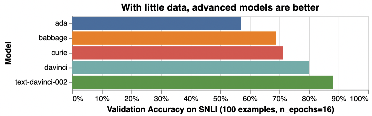
Below is an illustrative example of how adding training examples improves classification accuracy.
아래는 학습 예제를 추가하여 분류 정확도를 향상시키는 방법을 보여주는 예시입니다.
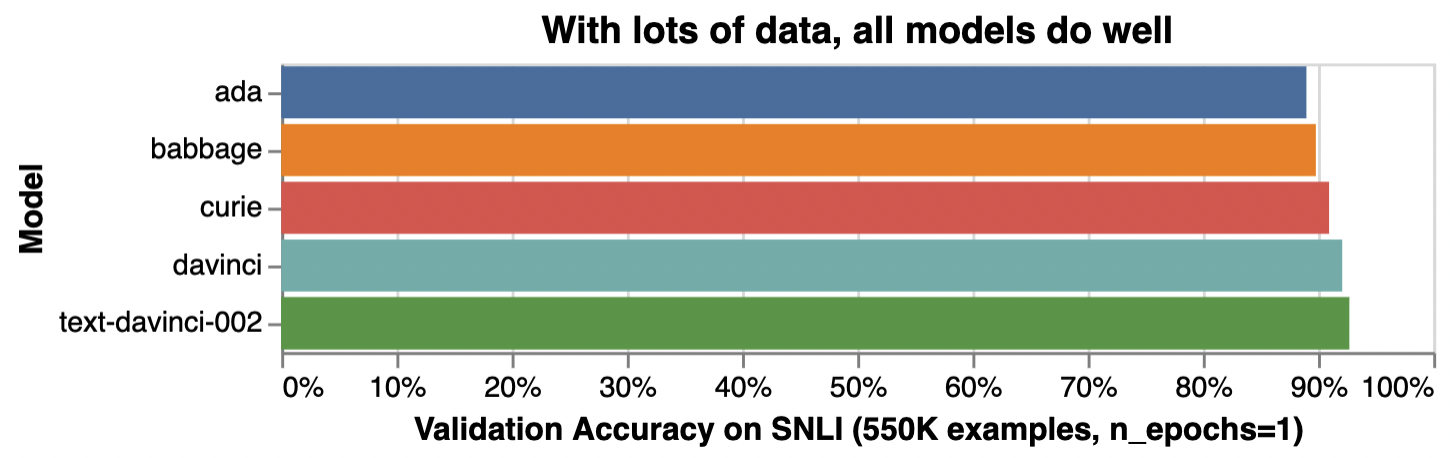
Illustrative examples of text classification performance on the Stanford Natural Language Inference (SNLI) Corpus, in which ordered pairs of sentences are classified by their logical relationship: either contradicted, entailed (implied), or neutral. Default fine-tuning parameters were used when not otherwise specified.
SNLI(Stanford Natural Language Inference) 코퍼스의 텍스트 분류 성능에 대한 예시로, 정렬된 문장 쌍이 논리적 관계(모순됨, 함축됨(암시됨) 또는 중립)에 따라 분류됩니다. 달리 지정되지 않은 경우 기본 fine-tuning 매개변수가 사용되었습니다.
Very roughly, we typically see that a few thousand examples are needed to get good performance:
아주 대략적으로 말해서 좋은 성능을 얻으려면 일반적으로 수천 개의 예제가 필요하다는 것을 알 수 있습니다.
Examples per label
Performance (rough estimate)
Hundreds
Decent
Thousands
Good
Tens of thousands or more
Great
To assess the value of getting more data, you can train models on subsets of your current dataset—e.g., 25%, 50%, 100%—and then see how performance scales with dataset size. If you plot accuracy versus number of training examples, the slope at 100% will indicate the improvement you can expect from getting more data. (Note that you cannot infer the value of additional data from the evolution of accuracy during a single training run, as a model half-trained on twice the data is not equivalent to a fully trained model.)
더 많은 데이터를 얻는 가치를 평가하기 위해 현재 데이터 세트의 하위 집합(예: 25%, 50%, 100%)에서 모델을 교육한 다음 데이터 세트 크기에 따라 성능이 어떻게 확장되는지 확인할 수 있습니다. 정확도 대 교육 예제 수를 플로팅하는 경우 100%의 기울기는 더 많은 데이터를 얻을 때 기대할 수 있는 개선을 나타냅니다. (두 배의 데이터로 절반만 훈련된 모델은 완전히 훈련된 모델과 동일하지 않기 때문에 단일 훈련 실행 동안 정확도의 진화에서 추가 데이터의 가치를 추론할 수 없습니다.)
How to evaluate your fine-tuned model
Evaluating your fine-tuned model is crucial to (a) improve your model and (b) tell when it’s good enough to be deployed.
fine-tuned 모델을 평가하는 것은 (a) 모델을 개선하고 (b) 언제 배포하기에 충분한 지를 알려주는 데 중요합니다.
Many metrics can be used to characterize the performance of a classifier
많은 메트릭을 사용하여 분류기의 성능을 특성화할 수 있습니다.
Accuracy
F1
Precision / Positive Predicted Value / False Discovery Rate
Recall / Sensitivity
Specificity
AUC / AUROC (area under the receiver operator characteristic curve)
AUPRC (area under the precision recall curve)
Cross entropy
Which metric to use depends on your specific application and how you weigh different types of mistakes. For example, if detecting something rare but consequential, where a false negative is costlier than a false positive, you might care about recall more than accuracy.
사용할 메트릭은 특정 응용 프로그램과 다양한 유형의 실수에 가중치를 두는 방법에 따라 다릅니다. 예를 들어 거짓 음성이 거짓 긍정보다 비용이 많이 드는 드물지만 결과적인 것을 감지하는 경우 정확도보다 리콜에 더 관심을 가질 수 있습니다.
The OpenAI API offers the option to calculate some of these classification metrics. If enabled, these metrics will be periodically calculated during fine-tuning as well as for your final model. You will see them as additional columns in your results file
OpenAI API는 이러한 분류 메트릭 중 일부를 계산하는 옵션을 제공합니다. 활성화된 경우 이러한 지표는 최종 모델뿐만 아니라 미세 조정 중에 주기적으로 계산됩니다. 결과 파일에 추가 열로 표시됩니다.
To enable classification metrics, you’ll need to:
분류 지표를 활성화하려면 다음을 수행해야 합니다.:
use single-token class labels
단일 토큰 클래스 레이블 사용
provide a validation file (same format as the training file)
유효성 검사 파일 제공(교육 파일과 동일한 형식)
set the flag --compute_classification_metrics
compute_classification_metrics 플래그 설정
for multiclass classification: set the argument --classification_n_classes
다중 클래스 분류: --classification_n_classes 인수 설정
for binary classification: set the argument --classification_positive_class
The following metrics are based on a classification threshold of 0.5 (i.e. when the probability is > 0.5, an example is classified as belonging to the positive class.)
다음 메트릭은 0.5의 분류 임계값을 기반으로 합니다(즉, 확률이 > 0.5인 경우 예는 포지티브 클래스에 속하는 것으로 분류됨).
classification/accuracy
classification/precision
classification/recall
classification/f{beta}
classification/auroc - AUROC
classification/auprc - AUPRC
Note that these evaluations assume that you are using text labels for classes that tokenize down to a single token, as described above. If these conditions do not hold, the numbers you get will likely be wrong.
이러한 평가에서는 위에서 설명한 대로 단일 토큰으로 토큰화하는 클래스에 대해 텍스트 레이블을 사용하고 있다고 가정합니다. 이러한 조건이 충족되지 않으면 얻은 숫자가 잘못되었을 수 있습니다.
Example outputs
Example metrics evolution over a training run, visualized with Weights & Biases
Weights & Biases로 시각화된 교육 실행에 대한 메트릭 진화의 예
How to pick the right model
OpenAI offers fine-tuning for 5 models: OpenAI는 fine-tuning에 다음 5가지 모델을 사용할 것을 권장합니다.
ada (cheapest and fastest)
babbage
curie
davinci
text-davinci-002 (highest quality)
Which model to use will depend on your use case and how you value quality versus price and speed.
사용할 모델은 사용 사례와 품질 대 가격 및 속도의 가치를 어떻게 평가하는지에 따라 달라집니다.
Generally, we see text classification use cases falling into two categories: simple and complex.
일반적으로 텍스트 분류 사용 사례는 단순과 복합의 두 가지 범주로 나뉩니다.
For tasks that are simple or straightforward, such as classifying sentiment, larger models offer diminishing benefit, as illustrated below:
감정 분류와 같이 간단하거나 직접적인 작업의 경우 더 큰 모델은 아래 그림과 같이 이점이 적습니다.
Model
Illustrative accuracy*
Training cost**
Inference cost**
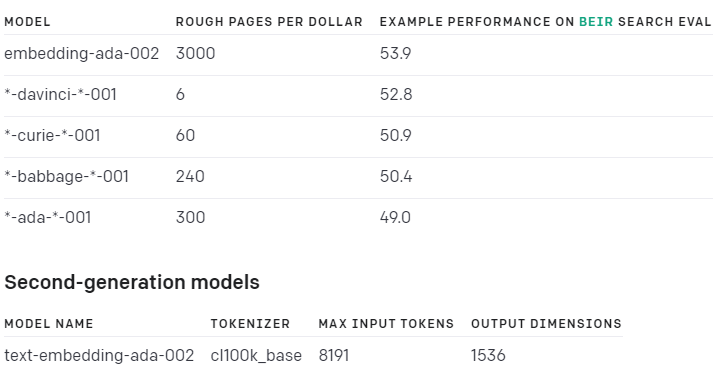
ada
89%
$0.0004 / 1K tokens (~3,000 pages per dollar)
$0.0016 / 1K tokens (~800 pages per dollar)
babbage
90%
$0.0006 / 1K tokens (~2,000 pages per dollar)
$0.0024 / 1K tokens (~500 pages per dollar)
curie
91%
$0.003 / 1K tokens (~400 pages per dollar)
$0.012 / 1K tokens (~100 pages per dollar)
davinci
92%
$0.03 / 1K tokens (~40 pages per dollar)
$0.12 / 1K tokens (~10 pages per dollar)
text-davinci-002
93%
unreleased
unreleased
*Illustrative accuracy on the SNLI dataset, in which sentence pairs are classified as contradictions, implications, or neutral
*문장 쌍이 모순, 암시 또는 중립으로 분류되는 SNLI 데이터 세트에 대한 설명 정확도
**Pages per dollar figures assume ~800 tokens per page. OpenAI Pricing.
Illustrative examples of text classification performance on the Stanford Natural Language Inference (SNLI) Corpus, in which ordered pairs of sentences are classified by their logical relationship: either contradicted, entailed (implied), or neutral. Default fine-tuning parameters were used when not otherwise specified.
SNLI(Stanford Natural Language Inference) 코퍼스의 텍스트 분류 성능에 대한 예시로, 정렬된 문장 쌍이 논리적 관계(모순됨, 함축됨(암시됨) 또는 중립)에 따라 분류됩니다. 달리 지정되지 않은 경우 기본 미세 조정 매개변수가 사용되었습니다.
For complex tasks, requiring subtle interpretation or reasoning or prior knowledge or coding ability, the performance gaps between models can be larger, and better models like curie or text-davinci-002 could be the best fit.
미묘한 해석이나 추론 또는 사전 지식이나 코딩 능력이 필요한 복잡한 작업의 경우 모델 간의 성능 차이가 더 클 수 있으며 curie 또는 text-davinci-002와 같은 더 나은 모델이 가장 적합할 수 있습니다.
A single project might end up trying all models. One illustrative development path might look like this:
단일 프로젝트에서 모든 모델을 시도하게 될 수 있습니다. 예시적인 개발 경로는 다음과 같습니다.
Test code using the cheapest & fastest model (ada)
가장 저렴하고 빠른 모델(ada)을 사용하여 테스트 코드
Run a few early experiments to check whether your dataset works as expected with a middling model (curie)
중간 모델(curie)에서 데이터 세트가 예상대로 작동하는지 확인하기 위해 몇 가지 초기 실험을 실행합니다.
Run a few more experiments with the best model to see how far you can push performance (text-davinci-002)
최상의 모델로 몇 가지 실험을 더 실행하여 성능을 얼마나 높일 수 있는지 확인하십시오(text-davinci-002).
Once you have good results, do a training run with all models to map out the price-performance frontier and select the model that makes the most sense for your use case (ada, babbage, curie, davinci, text-davinci-002)
좋은 결과를 얻으면 모든 모델로 교육 실행을 수행하여 가격 대비 성능 한계를 파악하고 사용 사례에 가장 적합한 모델(ada, babbage, curie, davinci, text-davinci-002)을 선택합니다.
Another possible development path that uses multiple models could be:
여러 모델을 사용하는 또 다른 가능한 개발 경로는 다음과 같습니다.
Starting with a small dataset, train the best possible model (text-davinci-002)
작은 데이터 세트로 시작하여 가능한 최상의 모델 훈련(text-davinci-002)
Use this fine-tuned model to generate many more labels and expand your dataset by multiples
이 미세 조정된 모델을 사용하여 더 많은 레이블을 생성하고 데이터 세트를 배수로 확장하십시오.
Use this new dataset to train a cheaper model (ada)
이 새로운 데이터 세트를 사용하여 더 저렴한 모델(ada) 훈련
How to pick training hyperparameters
Fine-tuning can be adjusted with various parameters. Typically, the default parameters work well and adjustments only result in small performance changes.
미세 조정은 다양한 매개변수로 조정할 수 있습니다. 일반적으로 기본 매개변수는 잘 작동하며 조정해도 성능이 약간만 변경됩니다.
Parameter
Default
Recommendation
n_epochs
controls how many times each example is trained on
각 예제가 훈련되는 횟수를 제어합니다.
4
For classification, we’ve seen good performance with numbers like 4 or 10. Small datasets may need more epochs and large datasets may need fewer epochs.
분류의 경우 4 또는 10과 같은 숫자로 좋은 성능을 보였습니다. 작은 데이터 세트에는 더 많은 에포크가 필요할 수 있고 큰 데이터 세트에는 더 적은 에포크가 필요할 수 있습니다.
If you see low training accuracy, try increasing n_epochs. If you see high training accuracy but low validation accuracy (overfitting), try lowering n_epochs.
훈련 정확도가 낮은 경우 n_epochs를 늘려 보십시오. 훈련 정확도는 높지만 검증 정확도(과적합)가 낮은 경우 n_epochs를 낮추십시오.
You can get training and validation accuracies by setting compute_classification_metrics to True and passing a validation file with labeled examples not in the training data. You can see graphs of these metrics evolving during fine-tuning with a Weights & Biases account.
compute_classification_metrics를 True로 설정하고 교육 데이터에 없는 레이블이 지정된 예제가 있는 유효성 검사 파일을 전달하여 교육 및 유효성 검사 정확도를 얻을 수 있습니다. Weights & Biases 계정을 사용하여 미세 조정하는 동안 진화하는 이러한 지표의 그래프를 볼 수 있습니다.
batch_size controls the number of training examples used in a single training pass 단일 교육 패스에 사용되는 교육 예제의 수를 제어합니다.
null (which dynamically adjusts to 0.2% of training set, capped at 256) (트레이닝 세트의 0.2%로 동적으로 조정되며 256으로 제한됨)
We’ve seen good performance in the range of 0.01% to 2%, but worse performance at 5%+. In general, larger batch sizes tend to work better for larger datasets.
우리는 0.01%에서 2% 범위에서 좋은 성능을 보았지만 5% 이상에서는 더 나쁜 성능을 보였습니다. 일반적으로 더 큰 배치 크기는 더 큰 데이터 세트에서 더 잘 작동하는 경향이 있습니다.
learning_rate_multiplier controls rate at which the model weights are updated 모델 가중치가 업데이트되는 속도를 제어합니다.
null (which dynamically adjusts to 0.05, 0.1, or 0.2 depending on batch size) (배치 크기에 따라 0.05, 0.1 또는 0.2로 동적으로 조정됨)
We’ve seen good performance in the range of 0.02 to 0.5. Larger learning rates tend to perform better with larger batch sizes.
0.02~0.5 범위에서 좋은 성능을 보였습니다. 더 큰 학습 속도는 더 큰 배치 크기에서 더 잘 수행되는 경향이 있습니다.
prompt_loss_weight controls how much the model learns from prompt tokens vs completion tokens 모델이 프롬프트 토큰과 완료 토큰에서 학습하는 양을 제어합니다.
0.1
If prompts are very long relative to completions, it may make sense to reduce this weight to avoid over-prioritizing learning the prompt. In our tests, reducing this to 0 is sometimes slightly worse or sometimes about the same, depending on the dataset.
프롬프트가 완료에 비해 매우 긴 경우 프롬프트 학습에 과도한 우선순위를 두지 않도록 이 가중치를 줄이는 것이 좋습니다. 테스트에서 데이터 세트에 따라 이를 0으로 줄이는 것이 때때로 약간 더 나쁘거나 거의 동일합니다.
More detail on prompt_loss_weight
When a model is fine-tuned, it learns to produce text it sees in both the prompt and the completion. In fact, from the point of view of the model being fine-tuned, the distinction between prompt and completion is mostly arbitrary. The only difference between prompt text and completion text is that the model learns less from each prompt token than it does from each completion token. This ratio is controlled by the prompt_loss_weight, which by default is 10%.
모델이 미세 조정되면 prompt and the completion 모두에 표시되는 텍스트를 생성하는 방법을 학습합니다. 실제로 미세 조정되는 모델의 관점에서 신속함과 완료의 구분은 대부분 임의적입니다. 프롬프트 텍스트와 완료 텍스트의 유일한 차이점은 모델이 각 완료 토큰에서 학습하는 것보다 각 프롬프트 토큰에서 학습하는 내용이 적다는 것입니다. 이 비율은 prompt_loss_weight에 의해 제어되며 기본적으로 10%입니다.
A prompt_loss_weight of 100% means that the model learns from prompt and completion tokens equally. In this scenario, you would get identical results with all training text in the prompt, all training text in the completion, or any split between them. For classification, we recommend against 100%.
100%의 prompt_loss_weight는 모델이 프롬프트 및 완료 토큰에서 동일하게 학습함을 의미합니다. 이 시나리오에서는 프롬프트의 모든 학습 텍스트, 완성의 모든 학습 텍스트 또는 이들 간의 분할에 대해 동일한 결과를 얻습니다. 분류의 경우 100% 대비를 권장합니다.
A prompt loss weight of 0% means that the model’s learning is focused entirely on the completion tokens. Note that even in this case, prompts are still necessary because they set the context for each completion. Sometimes we’ve seen a weight of 0% reduce classification performance slightly or make results slightly more sensitive to learning rate; one hypothesis is that a small amount of prompt learning helps preserve or enhance the model’s ability to understand inputs.
0%의 즉각적인 손실 가중치는 모델의 학습이 완료 토큰에 전적으로 집중되어 있음을 의미합니다. 이 경우에도 프롬프트는 각 완료에 대한 컨텍스트를 설정하기 때문에 여전히 필요합니다. 때때로 우리는 0%의 가중치가 분류 성능을 약간 감소시키거나 결과가 학습률에 약간 더 민감해지는 것을 보았습니다. 한 가지 가설은 소량의 즉각적인 학습이 입력을 이해하는 모델의 능력을 유지하거나 향상시키는 데 도움이 된다는 것입니다.
Example hyperparameter sweeps
n_epochs
The impact of additional epochs is particularly high here, because only 100 training examples were used.
100개의 학습 예제만 사용되었기 때문에 추가 에포크의 영향이 여기에서 특히 높습니다.
learning_rate_multiplier
prompt_loss_weight
How to pick inference parameters
Parameter
Recommendation
model
(discussed above) [add link]
temperature
Set temperature=0 for classification. Positive values add randomness to completions, which can be good for creative tasks but is bad for a short deterministic task like classification. 분류를 위해 온도=0으로 설정합니다. 양수 값은 완성에 임의성을 추가하므로 창의적인 작업에는 좋을 수 있지만 분류와 같은 짧은 결정론적 작업에는 좋지 않습니다.
max_tokens
If using single-token labels (or labels with unique first tokens), set max_tokens=1. If using longer labels, set to the length of your longest label. 단일 토큰 레이블(또는 고유한 첫 번째 토큰이 있는 레이블)을 사용하는 경우 max_tokens=1로 설정합니다. 더 긴 레이블을 사용하는 경우 가장 긴 레이블의 길이로 설정하십시오.
stop
If using labels of different length, you can optionally append a stop sequence like ‘ END’ to your training completions. Then, pass stop=‘ END’ in your inference call to prevent the model from generating excess text after appending short labels. (Otherwise, you can get completions like “burger -->” “ edible edible edible edible edible edible” as the model continues to generate output after the label is appended.) An alternative solution is to post-process the completions and look for prefixes that match any labels. 길이가 다른 레이블을 사용하는 경우 선택적으로 학습 완료에 ' END'와 같은 중지 시퀀스를 추가할 수 있습니다. 그런 다음 짧은 레이블을 추가한 후 모델이 과도한 텍스트를 생성하지 않도록 추론 호출에서 stop=' END'를 전달합니다. (그렇지 않으면 레이블이 추가된 후에도 모델이 계속 출력을 생성하므로 "burger -->" " edible edible edible edible edible"와 같은 완성을 얻을 수 있습니다.) 대체 솔루션은 완성을 후처리하고 접두사를 찾는 것입니다. 모든 레이블과 일치합니다.
logit_bias
If using single-token labels, set logit_bias={“label1”: 100, “label2”:100, …} with your labels in place of “label1” etc.
For tasks with little data or complex labels, models can output tokens for invented classes never specified in your training set. logit_bias can fix this by upweighting your label tokens so that illegal label tokens are never produced. If using logit_bias in conjunction with multi-token labels, take extra care to check how your labels are being split into tokens, as logit_bias only operates on individual tokens, not sequences.
데이터가 적거나 레이블이 복잡한 작업의 경우 모델은 훈련 세트에 지정되지 않은 발명된 클래스에 대한 토큰을 출력할 수 있습니다. logit_bias는 불법 레이블 토큰이 생성되지 않도록 레이블 토큰의 가중치를 높여 이 문제를 해결할 수 있습니다. 다중 토큰 레이블과 함께 logit_bias를 사용하는 경우 logit_bias는 시퀀스가 아닌 개별 토큰에서만 작동하므로 레이블이 토큰으로 분할되는 방식을 특히 주의하십시오.
Logit_bias can also be used to bias specific labels to appear more or less frequently. Logit_bias를 사용하여 특정 레이블이 더 자주 또는 덜 자주 표시되도록 바이어스할 수도 있습니다.
logprobs
Getting the probabilities of each label can be useful for computing confidence scores, precision-recall curves, calibrating debiasing using logit_bias, or general debugging. 각 레이블의 확률을 얻는 것은 신뢰도 점수 계산, 정밀도 재현 곡선, logit_bias를 사용한 편향성 보정 보정 또는 일반 디버깅에 유용할 수 있습니다.
Setting logprobs=5 will return, for each token position of the completion, the top 5 most likely tokens and the natural logs of their probabilities. To convert logprobs into probabilities, raise e to the power of the logprob (probability = e^logprob). The probabilities returned are independent of temperature and represent what the probability would have been if the temperature had been set to 1. By default 5 is the maximum number of logprobs returned, but exceptions can be requested by emailing support@openai.com and describing your use case.
logprobs=5로 설정하면 완료의 각 토큰 위치에 대해 가장 가능성이 높은 상위 5개 토큰과 해당 확률의 자연 로그가 반환됩니다. logprobs를 확률로 변환하려면 e를 logprob의 거듭제곱으로 올립니다(probability = e^logprob). 반환된 확률은 온도와 무관하며 온도가 1로 설정되었을 경우의 확률을 나타냅니다. 기본적으로 5는 반환되는 logprobs의 최대 수. 예외는 support@openai.com으로 이메일을 보내주세요 귀하의 사용 사례를 보내 주세요.
Example API call to get probabilities for the 5 most likely tokens 가능성이 가장 높은 5개의 토큰에 대한 확률을 얻기 위한 API 호출 예
api_response = openai.Completion.create( model="{fine-tuned model goes here, without brackets}", prompt="toothpaste -->", temperature=0, max_tokens=1, logprobs=5 ) dict_of_logprobs = api_response['choices'][0]['logprobs']['top_logprobs'][0].to_dict() dict_of_probs = {k: 2.718**v for k, v in dict_of_logprobs.items()}
echo
In cases where you want the probability of a particular label that isn’t showing up in the list of logprobs, the echo parameter is useful. If echo is set to True and logprobs is set to a number, the API response will include logprobs for every token of the prompt as well as the completion. So, to get the logprob for any particular label, append that label to the prompt and make an API call with echo=True, logprobs=0, and max_tokens=0.
logprobs 목록에 나타나지 않는 특정 레이블의 확률을 원하는 경우 echo 매개변수가 유용합니다. echo가 True로 설정되고 logprobs가 숫자로 설정되면 API 응답에는 완료뿐 아니라 프롬프트의 모든 토큰에 대한 logprobs가 포함됩니다. 따라서 특정 레이블에 대한 logprob를 가져오려면 해당 레이블을 프롬프트에 추가하고 echo=True, logprobs=0 및 max_tokens=0으로 API 호출을 수행합니다.
Example API call to get the logprobs of prompt tokens
For complex tasks that require reasoning, one useful technique you can experiment with is inserting explanations before the final answer. Giving the model extra time and space to think ‘aloud’ can increase the odds it arrives at the correct final answer.
추론이 필요한 복잡한 작업의 경우 실험할 수 있는 유용한 기술 중 하나는 최종 답변 앞에 설명을 삽입하는 것입니다. 모델에게 '큰 소리로' 생각할 수 있는 추가 시간과 공간을 제공하면 올바른 최종 답변에 도달할 가능성이 높아질 수 있습니다.
“Q: Where do you put your grapes just before checking out? Answer Choices: (a) mouth (b) grocery cart (c) supermarket (d) fruit basket (e) fruit market A:”
“(b)”
“The answer should be the place where grocery items are placed before checking out. Of the above choices, grocery cart makes the most sense for holding grocery items. Therefore, the answer is grocery cart (b).”
“답은 체크아웃하기 전에 식료품을 두는 장소여야 합니다. 위의 선택 중에서 식료품 카트는 식료품을 보관하는 데 가장 적합합니다. 따라서 정답은 식료품 카트(b)입니다.”
Although it can sound daunting to write many example explanations, it turns out you can use large language models to write the explanations. In 2022, Zelikman, Wu, et al. published a procedure called STaR (Self-Taught Reasoner) in which a few-shot prompt can be used to generate a set of {questions, rationales, answers} from just a set of {questions, answers}
많은 예제 설명을 작성하는 것이 어렵게 들릴 수 있지만 큰 언어 모델을 사용하여 설명을 작성할 수 있습니다. 2022년 Zelikman, Wu, et al. {질문, 답변} 세트에서 {질문, 근거, 답변} 세트를 생성하기 위해 몇 번의 프롬프트를 사용할 수 있는 STaR(Self-Taught Reasoner)라는 절차를 발표했습니다.
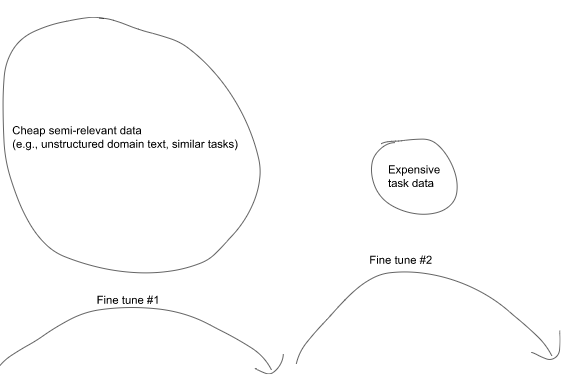
Sequential fine-tuning
Models can be fine-tuned sequentially as many times as you like. One way you can use this is to pre-train your model on a large amount of relevant text, such as unstructured domain text or similar classification tasks, and then afterwards fine-tune on examples of the task you want the model to perform. An example procedure could look like:
모델은 원하는 만큼 순차적으로 미세 조정할 수 있습니다. 이를 사용할 수 있는 한 가지 방법은 구조화되지 않은 도메인 텍스트 또는 유사한 분류 작업과 같은 많은 양의 관련 텍스트에 대해 모델을 사전 훈련한 다음 나중에 모델이 수행할 작업의 예를 미세 조정하는 것입니다. 예제 절차는 다음과 같습니다.
Step 1: Fine-tune on cheap, semi-relevant data
E.g., unstructured domain text (such as legal or medical text)
E.g., similar task data (such as another large classification set)
Step 2: Fine-tune on expensive labeled examples
E.g., text and classes (if training a classifier)
To fine-tune a previously fine-tuned model, pass in the fine-tuned model name when creating a new fine-tuning job (e.g. -m curie:ft-<org>-<date>). Other training parameters do not have to be changed, however if your new training data is much smaller than your previous training data, you may find it useful to reduce learning_rate_multiplier by a factor of 2 to 4.
이전에 미세 조정된 모델을 미세 조정하려면 새 미세 조정 작업을 생성할 때 미세 조정된 모델 이름을 전달합니다(예: -m curie:ft-<org>-<date>). 다른 훈련 매개변수는 변경할 필요가 없지만 새 훈련 데이터가 이전 훈련 데이터보다 훨씬 작은 경우 learning_rate_multiplier를 2~4배 줄이는 것이 유용할 수 있습니다.
Common mistakes
The most common mistakes when fine-tuning text classifiers are usually related to training data.
텍스트 분류기를 미세 조정할 때 가장 흔한 실수는 일반적으로 훈련 데이터와 관련이 있습니다.
Common mistake #1: Insufficiently specified training data
One thing to keep in mind is that training data is more than just a mapping of inputs to correct answers. Crucially, the inputs need to contain the information needed to derive an answer.
한 가지 명심해야 할 점은 교육 데이터가 정답에 대한 입력의 매핑 이상이라는 것입니다. 결정적으로 입력에는 답을 도출하는 데 필요한 정보가 포함되어야 합니다.
For example, consider fine-tuning a model to predict someone’s grades using the following dataset:
예를 들어 다음 데이터 세트를 사용하여 누군가의 성적을 예측하도록 모델을 미세 조정하는 것을 고려하십시오.
Prompt
Completion
“Alice >>>”
“ A”
“Bob >>>”
“ B+”
“Coco >>>”
“ A-”
“Dominic >>>”
“ B”
Prompt
Completion
“Esmeralda >>>”
???
Without knowing why these students got the grades they did, there is insufficient information for the model to learn from and no hope of making a good personalized prediction for Esmeralda.
이 학생들이 자신이 받은 성적을 받은 이유를 모르면 모델이 배울 수 있는 정보가 충분하지 않으며 Esmeralda에 대해 좋은 개인화된 예측을 할 수 있는 희망이 없습니다.
This can happen more subtly when some information is given but some is still missing. For example, if fine-tuning a classifier on whether a business expense is allowed or disallowed, and the business expense policy varies by date or by location or by employee type, make sure the input contains information on dates, locations, and employee type.
이것은 일부 정보가 제공되었지만 일부가 여전히 누락된 경우 더 미묘하게 발생할 수 있습니다. 예를 들어 비즈니스 비용이 허용되는지 여부에 대한 분류자를 미세 조정하고 비즈니스 비용 정책이 날짜, 위치 또는 직원 유형에 따라 달라지는 경우 입력에 날짜, 위치 및 직원 유형에 대한 정보가 포함되어 있는지 확인하십시오.
Prompt
Completion
“Amount: $50 Item: Steak dinner
###
”
“ allowed”
“Amount: $50 Item: Steak dinner
###
”
“ disallowed”
Prompt
Completion
“Amount: $50 Item: Steak dinner
###
”
???
Common mistake #2: Input data format that doesn’t match the training data format
Make sure that when you use your fine-tuned model, your submitted prompts match the format of your training data.
미세 조정된 모델을 사용할 때 제출된 프롬프트가 훈련 데이터의 형식과 일치하는지 확인하십시오.
Training data format
API call
OK?
“dog toy -->”
“dog toy”
❌Missing separator
“Amount: $50 Item: Steak dinner
###
”
“Is a $50 steak dinner allowed?
###
“
❌Different format
“Esmeralda >>>”
“Esmeralda >>> ”
❌Extra space appended
More examples
Below, we share more examples of training data for possible classifiers.
아래에서 가능한 분류기에 대한 훈련 데이터의 더 많은 예를 공유합니다.
Truthful consistency classifier
Prompt
Completion
"Company: BHFF insurance Product: allround insurance Ad: One stop shop for all your insurance needs! Supported:"
Product review classifier (with multiple classes labeled in parallel)
Prompt
Completion
"4/5 stars
Camera seems fine. Not amazing, but perfectly decent.
Biggest complaint is that the cable is only 5 feet long, which I didn't think to check. It's my fault, so I won't return it, but 5 feet is really short if you have multiple monitors and probably impossible if you have a desktop on the floor next to a standing desk.
###
Positives:"
“ fine, perfectly decent Negatives: not amazing, cable is only 5 feet long Overall sentiment: positive Possible improvements: longer cable Return risk: 1 Support priority: low Customer type: N/A”
"4/5 stars
I bought this on sale for $70. I'm satisfied with it.
(1) The instructions weren't that bad. (There was really only one ambiguous step, and it was easy to make an educated guess at the right way to go. Surprised by the ordering of one of the steps because some bars were hanging there for a while, but whatever.)
(2) It definitely is labor intensive - the most painful step is screwing in 24 small wood screws to get the hooks attached. And it takes a bit of skill to get them all vertically parallel. Got a big blister from all the screwing. And the angles made it hard to use power tools - ended up screwing in by hand because it was easier to stay vertical next to the hook.
(3) I weight 170 pounds and honestly the bench seems fine for supporting my weight. I was worried from the other reviews. But my trick was to leave things a little loose until the end and then really tighten everything once it was all together. I think really tightening at the end prevents any squeaky rocking. But only used it one day so far, so we'll see.
Overall this is definitely cheap, but feels totally fine. It's cheap in a cheap way, not cheap in a junky knockoff way. Would buy again. Looks great.
###
Positives:"
“ instructions weren’t that bad, looks great Negatives: ambiguous step, labor intensive, got a big blister, cheap Overall sentiment: positive Possible improvements: less ambiguous instructions Return risk: 0 Support priority: low Customer type: N/A”
"5/5 stars
I'm a fan. It's shiny and pure metal. Exactly what I wanted.
###
Positives:”
“ shiny, pure metal Negatives: N/A Overall sentiment: positive Possible improvements: N/A Return risk: 0 Support priority: low Customer type: N/A
Sentiment analyzer
Prompt
Completion
"Overjoyed with the new iPhone! ->"
“ positive”
"@lakers disappoint for a third straight night https://t.co/38EFe43 ->"
“ negative”
Email prioritizer
Prompt
Completion
"Subject: Update my address From: Joe Doe To: support@ourcompany.com Date: 2021-06-03 Content: Hi, I would like to update my billing address to match my delivery address.
Please let me know once done.
Thanks, Joe
###
"
“ 4”
Legal claim detector
Prompt
Completion
"When the IPV (injection) is used, 90% or more of individuals develop protective antibodies to all three serotypes of polio virus after two doses of inactivated polio vaccine (IPV), and at least 99% are immune to polio virus following three doses. -->"
“ efficacy”
"Jonas Edward Salk (/sɔːlk/; born Jonas Salk; October 28, 1914 – June 23, 1995) was an American virologist and medical researcher who developed one of the first successful polio vaccines. He was born in New York City and attended the City College of New York and New York University School of Medicine. -->"
“ not”
News subject detector
Prompt
Completion
"PC World - Upcoming chip set will include built-in security features for your PC. >>>"
“ 4”
(where 4 = Sci/Tech)
“Newspapers in Greece reflect a mixture of exhilaration that the Athens Olympics proved successful, and relief that they passed off without any major setback. >>>”
“ 2”
(where 2 = Sports)
Logical relationship detector
Prompt
Completion
"A land rover is being driven across a river. A vehicle is crossing a river.
###
"
“ implication”
"Violin soloists take the stage during the orchestra's opening show at the theater. People are playing the harmonica while standing on a roof.
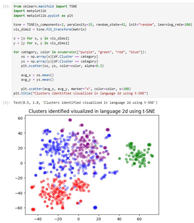
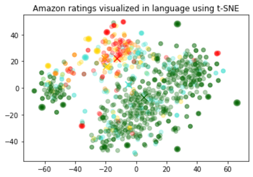
그리고 plt.title()에서 이 표의 제목을 정해주면 결과와 같은 그림을 얻을 수 있습니다.
4개의 그룹중에 녹색 그룹은 다른 그룹들과 좀 동떨어져 있는 것을 보실 수 있습니다.
2. Text samples in the clusters & naming the clusters
지금까지는 raw data를 clustering 하는 법과 이 clustering 한 데이터를 시각화 해서 보여주는 방법을 보았습니다.
이제 openai의 api를 이용해서 각 클러스터의 랜덤 샘플들을 보여 주는 코드입니다.
openai.Completion.create() api를 사용할 것이고 모델 (engine)은 text-ada-001을 사용합니다.
prompt는 아래 질문 입니다.
What do the following customer reviews have in common?
그러면 각 클러스터 별로 review 를 분석한 값들이 response 됩니다.
우선 아래 코드를 실행 해 보겠습니다.
import openai

def open_file(filepath):
    with open(filepath, 'r', encoding='utf-8') as infile:
        return infile.read()

openai.api_key = open_file('openaiapikey.txt')

# Reading a review which belong to each group.
rev_per_cluster = 5

for i in range(n_clusters):
    print(f"Cluster {i} Theme:", end=" ")

    reviews = "\n".join(
        df[df.Cluster == i]
        .combined.str.replace("Title: ", "")
        .str.replace("\n\nContent: ", ":  ")
        .sample(rev_per_cluster, random_state=42)
        .values
    )
    response = openai.Completion.create(
        engine="text-ada-001",  #"text-davinci-003",
        prompt=f'What do the following customer reviews have in common?\n\nCustomer reviews:\n"""\n{reviews}\n"""\n\nTheme:',
        temperature=0,
        max_tokens=64,
        top_p=1,
        frequency_penalty=0,
        presence_penalty=0,
    )
    print(response)
openai를 import 하고 openai api key를 제공하는 부분으로 시작합니다.
그리고 rev_per_cluster는 5로 합니다.
그 다음 for 문에서 n_clusters만큼 루프를 도는데 위에서 n_clusters는 4로 설정돼 있었습니다.
reviews에는 Title과 Content 내용을 넣는데 샘플로 5가지를 무작위로 뽑아서 넣습니다.
그리고 이 reviews 값을 prompt에 삽입해서 openai.Completion.create() api로 request 합니다.
그러면 이 prompt에 대한 response 가 response 변수에 담깁니다.
이 response 만 우선 출력해 보겠습니다.
Cluster 0 Theme: {
"choices": [
{
"finish_reason": "stop",
"index": 0,
"logprobs": null,
"text": " Customer reviews:gluten free, healthy bars, content:\n\nThe customer reviews have in common that they save money on Amazon by ordering by themselves by looking for gluten free healthy bars. The bars are also delicious."
}
],
"created": 1677191195,
"id": "cmpl-6nEKppB6SqCz07LYTcaktEAgq06hm",
"model": "text-ada-001",
"object": "text_completion",
"usage": {
"completion_tokens": 44,
"prompt_tokens": 415,
"total_tokens": 459
}
}
Cluster 1 Theme: {
"choices": [
{
"finish_reason": "stop",
"index": 0,
"logprobs": null,
"text": " Cat food\n\nMessy, undelicious, and possibly unhealthy."
}
],
"created": 1677191195,
"id": "cmpl-6nEKpGffRc2jyJB4gNtuCa09dG2GT",
"model": "text-ada-001",
"object": "text_completion",
"usage": {
"completion_tokens": 15,
"prompt_tokens": 529,
"total_tokens": 544
}
}
Cluster 2 Theme: {
"choices": [
{
"finish_reason": "stop",
"index": 0,
"logprobs": null,
"text": " Coffee\n\nThe customer's reviews have in common that they are among the best in the market, Rodeo Drive, and that the customer is able to enjoy their coffee half and half because they have an Amazon account."
}
],
"created": 1677191196,
"id": "cmpl-6nEKqxza0t8vGRAiK9K5RtCy3Gwbl",
"model": "text-ada-001",
"object": "text_completion",
"usage": {
"completion_tokens": 45,
"prompt_tokens": 443,
"total_tokens": 488
}
}
Cluster 3 Theme: {
"choices": [
{
"finish_reason": "stop",
"index": 0,
"logprobs": null,
"text": " Customer reviews of different brands of soda."
}
],
"created": 1677191196,
"id": "cmpl-6nEKqKuxe4CVJTV4GlIZ7vxe6F85o",
"model": "text-ada-001",
"object": "text_completion",
"usage": {
"completion_tokens": 8,
"prompt_tokens": 616,
"total_tokens": 624
}
}
이 respons를 보시면 각 Cluster 별로 응답을 받았습니다.
위에 for 문에서 각 클러스터별로 request를 했기 때문입니다.
이제 이 중에서 실제 질문에 대한 답변인 choices - text 부분만 뽑아 보겠습니다.
import openai

def open_file(filepath):
    with open(filepath, 'r', encoding='utf-8') as infile:
        return infile.read()

openai.api_key = open_file('openaiapikey.txt')

# Reading a review which belong to each group.
rev_per_cluster = 5

for i in range(n_clusters):
    print(f"Cluster {i} Theme:", end=" ")

    reviews = "\n".join(
        df[df.Cluster == i]
        .combined.str.replace("Title: ", "")
        .str.replace("\n\nContent: ", ":  ")
        .sample(rev_per_cluster, random_state=42)
        .values
    )
    response = openai.Completion.create(
        engine="text-ada-001",  #"text-davinci-003",
        prompt=f'What do the following customer reviews have in common?\n\nCustomer reviews:\n"""\n{reviews}\n"""\n\nTheme:',
        temperature=0,
        max_tokens=64,
        top_p=1,
        frequency_penalty=0,
        presence_penalty=0,
    )

    print(response["choices"][0]["text"].replace("\n", ""))
답변은 아래와 같습니다.
Cluster 0 Theme:  Customer reviews:gluten free, healthy bars, content:The customer reviews have in common that they save money on Amazon by ordering by themselves by looking for gluten free healthy bars. The bars are also delicious.
Cluster 1 Theme:  Cat foodMessy, undelicious, and possibly unhealthy.
Cluster 2 Theme:  CoffeeThe customer's reviews have in common that they are among the best in the market, Rodeo Drive, and that the customer is able to enjoy their coffee half and half because they have an Amazon account.
Cluster 3 Theme:  Customer reviews of different brands of soda.
Cluster 0 Theme:      Unnamed: 0   ProductId          UserId  Score  \
117         400  B008JKU2CO  A1XV4W7JWX341C      5
25          274  B008JKTH2A  A34XBAIFT02B60      1
722         534  B0064KO16O  A1K2SU61D7G41X      5
289           7  B001KP6B98   ABWCUS3HBDZRS      5
590         948  B008GG2N2S  A1CLUIIJL6EHLU      5

                                               Summary  \
117  Loved these gluten free healthy bars, saved $$...
25   Should advertise coconut as an ingredient more...
722                                        very good!!
289                                  Excellent product
590                                          delicious

                                                  Text  \
117  These Kind Bars are so good and healthy & glut...
25   First, these should be called Mac - Coconut ba...
722  just like the runts<br />great flavor, def wor...
289  After scouring every store in town for orange ...
590  Gummi Frogs have been my favourite candy that ...

                                              combined  n_tokens  \
117  Title: Loved these gluten free healthy bars, s...        96
25   Title: Should advertise coconut as an ingredie...        78
722  Title: very good!!; Content: just like the run...        43
289  Title: Excellent product; Content: After scour...       100
590  Title: delicious; Content: Gummi Frogs have be...        75

                                             embedding  Cluster
117  [-0.002289338270202279, -0.01313735730946064, ...        0
25   [-0.01757248118519783, -8.266511576948687e-05,...        0
722  [-0.011768403463065624, -0.025617636740207672,...        0
289  [0.0007493243319913745, -0.017031244933605194,...        0
590  [-0.005802689120173454, 0.0007485789828933775,...        0
Cluster 1 Theme:      Unnamed: 0   ProductId          UserId  Score  \
536         731  B0029NIBE8  A3RKYD8IUC5S0N      2
332         184  B000WFRUOC   A22RVTZEIVHZA      4
424         153  B0007A0AQW  A15X1BO4CLBN3C      5
298          24  B003R0LKRW  A1OQSU5KYXEEAE      1
960         589  B003194PBC  A2FSDQY5AI6TNX      5

                              Summary  \
536  Messy and apparently undelicious
332                  The cats like it
424          cant get enough of it!!!
298               Food Caused Illness
960          My furbabies LOVE these!

                                                  Text  \
536  My cat is not a huge fan. Sure, she'll lap up ...
332  My 7 cats like this food but it is a little yu...
424  Our lil shih tzu puppy cannot get enough of it...
298  I switched my cats over from the Blue Buffalo ...
960  Shake the container and they come running. Eve...

                                              combined  n_tokens  \
536  Title: Messy and apparently undelicious; Conte...       181
332  Title: The cats like it; Content: My 7 cats li...        87
424  Title: cant get enough of it!!!; Content: Our ...        59
298  Title: Food Caused Illness; Content: I switche...       131
960  Title: My furbabies LOVE these!; Content: Shak...        47

                                             embedding  Cluster
536  [-0.002376032527536154, -0.0027701142244040966...        1
332  [0.02162935584783554, -0.011174295097589493, -...        1
424  [-0.007517425809055567, 0.0037251529283821583,...        1
298  [-0.0011128562036901712, -0.01970377005636692,...        1
960  [-0.009749102406203747, -0.0068712360225617886...        1
Cluster 2 Theme:      Unnamed: 0   ProductId          UserId  Score  \
135         410  B007Y59HVM  A2ERWXZEUD6APD      5
439         812  B0001UK0CM  A2V8WXAFG1TEOC      5
326         107  B003VXFK44  A21VWSCGW7UUAR      4
475         852  B000I6MCSY   AO34Q3JGZU0JQ      5
692         922  B003TC7WN4  A3GFZIL1E0Z5V8      5

                               Summary  \
135                  Fog Chaser Coffee
439                    Excellent taste
326   Good, but not Wolfgang Puck good
475             Just My Kind of Coffee
692  Rodeo Drive is Crazy Good Coffee!

                                                  Text  \
135  This coffee has a full body and a rich taste. ...
439  This is to me a great coffee, once you try it ...
326  Honestly, I have to admit that I expected a li...
475  Coffee Masters Hazelnut coffee used to be carr...
692  Rodeo Drive is my absolute favorite and I'm re...

                                              combined  n_tokens  \
135  Title: Fog Chaser Coffee; Content: This coffee...        42
439  Title: Excellent taste; Content: This is to me...        31
326  Title: Good, but not Wolfgang Puck good; Conte...       178
475  Title: Just My Kind of Coffee; Content: Coffee...       118
692  Title: Rodeo Drive is Crazy Good Coffee!; Cont...        59

                                             embedding  Cluster
135  [0.006498195696622133, 0.006776264403015375, 0...        2
439  [0.0039436533115804195, -0.005451332312077284,...        2
326  [-0.003140551969408989, -0.009995664469897747,...        2
475  [0.010913548991084099, -0.014923149719834328, ...        2
692  [-0.029914353042840958, -0.007755572907626629,...        2
Cluster 3 Theme:      Unnamed: 0   ProductId          UserId  Score  \
495         831  B0014X5O1C   AHYRTWABDAG1H      5
978         642  B00264S63G  A36AUU1UNRS48G      5
916         686  B008PYVINQ  A1DRWYIO7JN1MD      2
696         926  B0062P9XPU  A33KQALCZGXG8C      5
491         828  B000EIE20M  A39QHSDUBR8L0T      3

                               Summary  \
495  Wonderful alternative to soda pop
978      So convenient, for so little!
916                    bot very cheesy
696                         Delicious!
491                            Just ok

                                                  Text  \
495  This is a wonderful alternative to soda pop.  ...
978  I needed two vanilla beans for the Love Goddes...
916  Got this about a month ago.first of all it sme...
696  I am not a huge beer lover.  I do enjoy an occ...
491  I bought this brand because it was all they ha...

                                              combined  n_tokens  \
495  Title: Wonderful alternative to soda pop; Cont...       273
978  Title: So convenient, for so little!; Content:...       121
916  Title: bot very cheesy; Content: Got this abou...        46
696  Title: Delicious!; Content: I am not a huge be...        97
491  Title: Just ok; Content: I bought this brand b...        58

                                             embedding  Cluster
495  [0.022326279431581497, -0.018449820578098297, ...        3
978  [-0.004598899278789759, -0.01737511157989502, ...        3
916  [-0.010750919580459595, -0.0193503275513649, -...        3
696  [0.009483409114181995, -0.017691848799586296, ...        3
491  [-0.0023960231337696314, -0.006881058216094971...        3
여기서 데이터를 아래와 같이 가공을 합니다.
    for j in range(rev_per_cluster):
        print(sample_cluster_rows.Score.values[j], end=", ")
        print(sample_cluster_rows.Summary.values[j], end=":   ")
        print(sample_cluster_rows.Text.str[:70].values[j])
Score의 값들을 가지고 오고 끝에는 쉼표 , 를 붙입니다.
그리고 Summary의 값을 가지고 오고 끝에는 : 를 붙입니다.
그리고 Text컬럼의 string을 가지고 오는데 70자 까지만 가지고 옵니다.
전체 결과를 보겠습니다.
Cluster 0 Theme:  Customer reviews:gluten free, healthy bars, content:The customer reviews have in common that they save money on Amazon by ordering by themselves by looking for gluten free healthy bars. The bars are also delicious.
5, Loved these gluten free healthy bars, saved $$ ordering on Amazon:   These Kind Bars are so good and healthy & gluten free.  My daughter ca
1, Should advertise coconut as an ingredient more prominently:   First, these should be called Mac - Coconut bars, as Coconut is the #2
5, very good!!:   just like the runts<br />great flavor, def worth getting<br />I even o
5, Excellent product:   After scouring every store in town for orange peels and not finding an
5, delicious:   Gummi Frogs have been my favourite candy that I have ever tried. of co
Cluster 1 Theme:  Cat foodMessy, undelicious, and possibly unhealthy.
2, Messy and apparently undelicious:   My cat is not a huge fan. Sure, she'll lap up the gravy, but leaves th
4, The cats like it:   My 7 cats like this food but it is a little yucky for the human. Piece
5, cant get enough of it!!!:   Our lil shih tzu puppy cannot get enough of it. Everytime she sees the
1, Food Caused Illness:   I switched my cats over from the Blue Buffalo Wildnerness Food to this
5, My furbabies LOVE these!:   Shake the container and they come running. Even my boy cat, who isn't
Cluster 2 Theme:  CoffeeThe customer's reviews have in common that they are among the best in the market, Rodeo Drive, and that the customer is able to enjoy their coffee half and half because they have an Amazon account.
5, Fog Chaser Coffee:   This coffee has a full body and a rich taste. The price is far below t
5, Excellent taste:   This is to me a great coffee, once you try it you will enjoy it, this
4, Good, but not Wolfgang Puck good:   Honestly, I have to admit that I expected a little better. That's not
5, Just My Kind of Coffee:   Coffee Masters Hazelnut coffee used to be carried in a local coffee/pa
5, Rodeo Drive is Crazy Good Coffee!:   Rodeo Drive is my absolute favorite and I'm ready to order more!  That
Cluster 3 Theme:  Customer reviews of different brands of soda.
5, Wonderful alternative to soda pop:   This is a wonderful alternative to soda pop.  It's carbonated for thos
5, So convenient, for so little!:   I needed two vanilla beans for the Love Goddess cake that my husbands
2, bot very cheesy:   Got this about a month ago.first of all it smells horrible...it tastes
5, Delicious!:   I am not a huge beer lover.  I do enjoy an occasional Blue Moon (all o
3, Just ok:   I bought this brand because it was all they had at Ranch 99 near us. I
이제 좀 보기 좋게 됐습니다.
이번 예제는 raw 데이터를 파이썬의 여러 모듈들을 이용해서 clustering을 하고 이 cluster별로 openai.Completion.create() api를 이용해서 궁금한 답을 받는 일을 하는 예제를 배웠습니다.
큰 raw data를 카테고리화 해서 나누고 이에 대한 summary나 기타 정보를 Completion api를 통해 얻을 수 있는 방법입니다.
전체 소스코드는 아래와 같습니다.
# imports
import numpy as np
import pandas as pd
# load data
datafile_path = "./data/fine_food_reviews_with_embeddings_1k.csv"
df = pd.read_csv(datafile_path)
df["embedding"] = df.embedding.apply(eval).apply(np.array) # convert string to numpy array
matrix = np.vstack(df.embedding.values)
matrix.shape
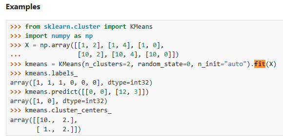
from sklearn.cluster import KMeans
n_clusters = 4
kmeans = KMeans(n_clusters=n_clusters, init="k-means++", random_state=42)
kmeans.fit(matrix)
labels = kmeans.labels_
df["Cluster"] = labels
df.groupby("Cluster").Score.mean().sort_values()
from sklearn.manifold import TSNE
import matplotlib
import matplotlib.pyplot as plt
tsne = TSNE(n_components=2, perplexity=15, random_state=42, init="random", learning_rate=200)
vis_dims2 = tsne.fit_transform(matrix)
x = [x for x, y in vis_dims2]
y = [y for x, y in vis_dims2]
for category, color in enumerate(["purple", "green", "red", "blue"]):
xs = np.array(x)[df.Cluster == category]
ys = np.array(y)[df.Cluster == category]
plt.scatter(xs, ys, color=color, alpha=0.3)
avg_x = xs.mean()
avg_y = ys.mean()
plt.scatter(avg_x, avg_y, marker="x", color=color, s=100)
plt.title("Clusters identified visualized in language 2d using t-SNE")
import openai
def open_file(filepath):
with open(filepath, 'r', encoding='utf-8') as infile:
return infile.read()
openai.api_key = open_file('openaiapikey.txt')
# Reading a review which belong to each group.
rev_per_cluster = 5
for i in range(n_clusters):
print(f"Cluster {i} Theme:", end=" ")
reviews = "\n".join(
df[df.Cluster == i]
.combined.str.replace("Title: ", "")
.str.replace("\n\nContent: ", ": ")
.sample(rev_per_cluster, random_state=42)
.values
)
response = openai.Completion.create(
engine="text-ada-001", #"text-davinci-003",
prompt=f'What do the following customer reviews have in common?\n\nCustomer reviews:\n"""\n{reviews}\n"""\n\nTheme:',
temperature=0,
max_tokens=64,
top_p=1,
frequency_penalty=0,
presence_penalty=0,
)
print(response["choices"][0]["text"].replace("\n", ""))
sample_cluster_rows = df[df.Cluster == i].sample(rev_per_cluster, random_state=42)
for j in range(rev_per_cluster):
print(sample_cluster_rows.Score.values[j], end=", ")
print(sample_cluster_rows.Summary.values[j], end=": ")
print(sample_cluster_rows.Text.str[:70].values[j])
이 예제의 training data는 [text_1, text_2, label] 형식 입니다.
두 쌍이 유사하면 레이블은 +1 이고 유사하지 않으면 -1 입니다.
output은 임베딩을 multiply 하는데 사용할 수 있는 matrix 입니다.
임베딩 multiplication을 통해서 좀 더 성능이 좋은 custom embedding을 얻을 수 있습니다.
그 다음 예제는 SNLI corpus에서 가지고 온 1000개의 sentence pair들을 사용합니다. 이 두 쌍은 논리적으로 연관돼 있는데 한 문장이 다른 문장을 암시하는 식 입니다. 논리적으로 연관 돼 있으면 레이블이 positive 입니다. 논리적으로 연관이 별로 없어 보이는 쌍은 레이블이 negative 가 됩니다.
그리고 clustering을 사용하는 경우에는 같은 클러스터 내의 텍스트 들로부터 한 쌍을 만듦으로서 positive 한 것을 생성할 수 있습니다. 그리고 다른 클러스터의 문장들로 쌍을 이루어서 negative를 생성할 수 있습니다.
다른 데이터 세트를 사용하면 100개 미만의 training example들 만으로도 좋은 성능 개선을 이루는 것을 볼 수 있었습니다. 물론 더 많은 예제를 사용하면 더 좋아지겠죠.
이제 소스 코드로 들어가 보겠습니다.
0. Imports
# imports
from typing import List, Tuple  # for type hints

import numpy as np  # for manipulating arrays
import pandas as pd  # for manipulating data in dataframes
import pickle  # for saving the embeddings cache
import plotly.express as px  # for plots
import random  # for generating run IDs
from sklearn.model_selection import train_test_split  # for splitting train & test data
import torch  # for matrix optimization

from openai.embeddings_utils import get_embedding, cosine_similarity  # for embeddings
# input parameters
embedding_cache_path = "data/snli_embedding_cache.pkl"  # embeddings will be saved/loaded here
default_embedding_engine = "babbage-similarity"  # choice of: ada, babbage, curie, davinci
num_pairs_to_embed = 1000  # 1000 is arbitrary - I've gotten it to work with as little as ~100
local_dataset_path = "data/snli_1.0_train_2k.csv"  # download from: https://nlp.stanford.edu/projects/snli/


def process_input_data(df: pd.DataFrame) -> pd.DataFrame:
    # you can customize this to preprocess your own dataset
    # output should be a dataframe with 3 columns: text_1, text_2, label (1 for similar, -1 for dissimilar)
    df["label"] = df["gold_label"]
    df = df[df["label"].isin(["entailment"])]
    df["label"] = df["label"].apply(lambda x: {"entailment": 1, "contradiction": -1}[x])
    df = df.rename(columns={"sentence1": "text_1", "sentence2": "text_2"})
    df = df[["text_1", "text_2", "label"]]
    df = df.head(num_pairs_to_embed)
    return df
여기서 하는 일은 cache 에 있는 데이터를 저장할 pkl 파일을 정하고 사용할 openai 모델을 정했습니다.
그리고 num_pairs_to_embed 변수에 1000을 할당했고 소스 데이터를 local_dataset_path 에 할당했습니다.
다음에 process_input_data() 함수가 나오는데요.
pandas 의 DataFrame 형식의 입력값을 받아서 처리한 다음에 다시 DataFrame형식으로 반환합니다.
대개 컬럼 이름들을 바꾸는 거네요.
그리고 DataFrame의 데이터를 1000 (num_pairs_to_embed) 개만 추려서 return 합니다.
2. Load and process input data
# load data
df = pd.read_csv(local_dataset_path)

# process input data
df = process_input_data(df)  # this demonstrates training data containing only positives

# view data
df.head()
이제 파일을 열고 위에 만들었던 함수를 통해 처리한 다음 상위 5개를 출력합니다.
df.head() 는 디폴트로 5개를 출력합니다. head() 안에 숫자를 넣으면 그 숫자만큼 출력합니다.
이걸 출력하면 이렇게 됩니다.
3. Split data into training test sets
synethetic negatives나 synethetic positives를 생성하기 전에 데이터를 training과 test sets 들로 구분하는 것은 아주 중요합니다.
training data의 text 문자열이 test data에 표시되는 것을 원하지 않을 겁니다.
contamination이 있는 경우 실제 production 보다 test metrics가 더 좋아 보일 수 있습니다.
# split data into train and test sets
test_fraction = 0.5  # 0.5 is fairly arbitrary
random_seed = 123  # random seed is arbitrary, but is helpful in reproducibility
train_df, test_df = train_test_split(
    df, test_size=test_fraction, stratify=df["label"], random_state=random_seed
)
train_df.loc[:, "dataset"] = "train"
test_df.loc[:, "dataset"] = "test"
여기에서는 sklearn.model_selection 모듈의 train_test_split() 함수를 사용해서 데이터를 training test sets로 분리 합니다.
4. Generate synthetic negatives
다음은 use case에 맞도록 수정해야 할 필요가 있을 수 있는 코드 입니다.
positives와 negarives 가 있는 데이터를 가지고 있을 경우 건너뛰어도 됩니다.
근데 만약 positives 한 데이터만 가지고 있다면 이 코드를 사용해야 할 것입니다.
이 코드 블록은 negatives 만 생성할 것입니다.
만약 여러분이 multiclass data를 가지고 있다면 여러분은 positives와 negatives 모두를 생성하기를 원할 겁니다.
positives는 레이블들을 공유하는 텍스트로 된 쌍이 될 수 있고 negatives는 레이블을 공유하지 않는 텍스트로 된 쌍이 될 수 있습니다.
최종 결과물은 text pair로 된 DataFrame이 될 것입니다. 각 쌍은 -1이나 1이 될 것입니다.
# generate negatives
def dataframe_of_negatives(dataframe_of_positives: pd.DataFrame) -> pd.DataFrame:
    """Return dataframe of negative pairs made by combining elements of positive pairs."""
    texts = set(dataframe_of_positives["text_1"].values) | set(
        dataframe_of_positives["text_2"].values
    )
    all_pairs = {(t1, t2) for t1 in texts for t2 in texts if t1 < t2}
    positive_pairs = set(
        tuple(text_pair)
        for text_pair in dataframe_of_positives[["text_1", "text_2"]].values
    )
    negative_pairs = all_pairs - positive_pairs
    df_of_negatives = pd.DataFrame(list(negative_pairs), columns=["text_1", "text_2"])
    df_of_negatives["label"] = -1
    return df_of_negatives
negatives_per_positive = (
    1  # it will work at higher values too, but more data will be slower
)
# generate negatives for training dataset
train_df_negatives = dataframe_of_negatives(train_df)
train_df_negatives["dataset"] = "train"
# generate negatives for test dataset
test_df_negatives = dataframe_of_negatives(test_df)
test_df_negatives["dataset"] = "test"
# sample negatives and combine with positives
train_df = pd.concat(
    [
        train_df,
        train_df_negatives.sample(
            n=len(train_df) * negatives_per_positive, random_state=random_seed
        ),
    ]
)
test_df = pd.concat(
    [
        test_df,
        test_df_negatives.sample(
            n=len(test_df) * negatives_per_positive, random_state=random_seed
        ),
    ]
)

df = pd.concat([train_df, test_df])
5. Calculate embeddings and cosine similarities
아래 코드 블럭에서는 임베딩을 저장하기 위한 캐시를 생성합니다.
이렇게 저장함으로서 다시 임베딩을 얻기 위해 openai api를 호출하면서 비용을 지불하지 않아도 됩니다.
# establish a cache of embeddings to avoid recomputing
# cache is a dict of tuples (text, engine) -> embedding
try:
    with open(embedding_cache_path, "rb") as f:
        embedding_cache = pickle.load(f)
except FileNotFoundError:
    precomputed_embedding_cache_path = "https://cdn.openai.com/API/examples/data/snli_embedding_cache.pkl"
    embedding_cache = pd.read_pickle(precomputed_embedding_cache_path)


# this function will get embeddings from the cache and save them there afterward
def get_embedding_with_cache(
    text: str,
    engine: str = default_embedding_engine,
    embedding_cache: dict = embedding_cache,
    embedding_cache_path: str = embedding_cache_path,
) -> list:
    print(f"Getting embedding for {text}")
    if (text, engine) not in embedding_cache.keys():
        # if not in cache, call API to get embedding
        embedding_cache[(text, engine)] = get_embedding(text, engine)
        # save embeddings cache to disk after each update
        with open(embedding_cache_path, "wb") as embedding_cache_file:
            pickle.dump(embedding_cache, embedding_cache_file)
    return embedding_cache[(text, engine)]


# create column of embeddings
for column in ["text_1", "text_2"]:
    df[f"{column}_embedding"] = df[column].apply(get_embedding_with_cache)

# create column of cosine similarity between embeddings
df["cosine_similarity"] = df.apply(
    lambda row: cosine_similarity(row["text_1_embedding"], row["text_2_embedding"]),
    axis=1,
)
6. Plot distribution of cosine similarity
이 예제에서는 cosine similarity를 사용하여 텍스트의 유사성을 측정합니다. openai 측의 경험상 대부분의 distance functions (L1, L2, cosine similarity)들은 모두 동일하게 작동한다고 합니다. 임베딩 값은 length 가 1로 정규화 되어 있기 때문에 임베딩에서 cosine similarity는 python의 numpy.dot() 과 동일한 결과를 내 놓습니다.
그래프들은 유사한 쌍과 유사하지 않은 쌍에 대한 cosine similarity 분포 사이에 겹치는 정도를 보여 줍니다. 겹치는 부분이 많다면 다른 유사한 쌍보다 cosine similarity가 크고 유사하지 않은 쌍이 많다는 의미 입니다.
계산의 정확도는 cosine similarity의 특정 임계치인 X 보다 크면 similar (1)을 예측하고 그렇치 않으면 dissimilar (0)을 예측합니다.
# calculate accuracy (and its standard error) of predicting label=1 if similarity>x
# x is optimized by sweeping from -1 to 1 in steps of 0.01
def accuracy_and_se(cosine_similarity: float, labeled_similarity: int) -> Tuple[float]:
    accuracies = []
    for threshold_thousandths in range(-1000, 1000, 1):
        threshold = threshold_thousandths / 1000
        total = 0
        correct = 0
        for cs, ls in zip(cosine_similarity, labeled_similarity):
            total += 1
            if cs > threshold:
                prediction = 1
            else:
                prediction = -1
            if prediction == ls:
                correct += 1
        accuracy = correct / total
        accuracies.append(accuracy)
    a = max(accuracies)
    n = len(cosine_similarity)
    standard_error = (a * (1 - a) / n) ** 0.5  # standard error of binomial
    return a, standard_error


# check that training and test sets are balanced
px.histogram(
    df,
    x="cosine_similarity",
    color="label",
    barmode="overlay",
    width=500,
    facet_row="dataset",
).show()

for dataset in ["train", "test"]:
    data = df[df["dataset"] == dataset]
    a, se = accuracy_and_se(data["cosine_similarity"], data["label"])
    print(f"{dataset} accuracy: {a:0.1%} ± {1.96 * se:0.1%}")
여기까지 작성한 코드를 실행 해 봤습니다.
처음엔 아래 내용을 출력하더니......
그 다음은 아래와 같은 형식으로 한도 끝도 없이 출력 하더라구요.
문서에 총 1만줄이 있던데 한줄 한줄 다 처리하느라 시간이 굉장히 많이 걸릴 것 같습니다.
전 3179 줄까지 출력한 후 시간이 너무 걸려서 강제로 중단 했습니다.
저는 text-embedding-ada-002 모델을 사용했습니다.
1천개의 토큰당 0.0004불이 과금 되는데 여기까지 저는 0.01불 즉 1센트가 과금 됐습니다.
그러면 0.01 / 0.0004 를 하니까 2만 5천 토큰 정도 사용 했나 보네요.
1만줄을 전부 다 하면 한 5센트 이내로 부과 되겠네요.
하여간 시간도 많이 걸리고 과금도 비교적 많이 되니 실행은 마지막에 딱 한번만 해 보기로 하겠습니다.
예제 상에는 6 Plot distribution of cosine similarity 에 있는 코드를 실행하면 아래와 같이 나온다고 합니다.
7. Optimize the matrix using the training data provided
def optimize_matrix(
modified_embedding_length: int = 2048, # in my brief experimentation, bigger was better (2048 is length of babbage encoding)
batch_size: int = 100,
max_epochs: int = 100,
learning_rate: float = 100.0, # seemed to work best when similar to batch size - feel free to try a range of values
dropout_fraction: float = 0.0, # in my testing, dropout helped by a couple percentage points (definitely not necessary)
df: pd.DataFrame = df,
print_progress: bool = True,
save_results: bool = True,
) -> torch.tensor:
"""Return matrix optimized to minimize loss on training data."""
run_id = random.randint(0, 2 ** 31 - 1) # (range is arbitrary)
# convert from dataframe to torch tensors
# e is for embedding, s for similarity label
def tensors_from_dataframe(
df: pd.DataFrame,
embedding_column_1: str,
embedding_column_2: str,
similarity_label_column: str,
) -> Tuple[torch.tensor]:
e1 = np.stack(np.array(df[embedding_column_1].values))
e2 = np.stack(np.array(df[embedding_column_2].values))
s = np.stack(np.array(df[similarity_label_column].astype("float").values))
e1 = torch.from_numpy(e1).float()
e2 = torch.from_numpy(e2).float()
s = torch.from_numpy(s).float()
return e1, e2, s
e1_train, e2_train, s_train = tensors_from_dataframe(
df[df["dataset"] == "train"], "text_1_embedding", "text_2_embedding", "label"
)
e1_test, e2_test, s_test = tensors_from_dataframe(
df[df["dataset"] == "train"], "text_1_embedding", "text_2_embedding", "label"
)
# create dataset and loader
dataset = torch.utils.data.TensorDataset(e1_train, e2_train, s_train)
train_loader = torch.utils.data.DataLoader(
dataset, batch_size=batch_size, shuffle=True
)
# define model (similarity of projected embeddings)
def model(embedding_1, embedding_2, matrix, dropout_fraction=dropout_fraction):
e1 = torch.nn.functional.dropout(embedding_1, p=dropout_fraction)
e2 = torch.nn.functional.dropout(embedding_2, p=dropout_fraction)
modified_embedding_1 = e1 @ matrix # @ is matrix multiplication
modified_embedding_2 = e2 @ matrix
similarity = torch.nn.functional.cosine_similarity(
modified_embedding_1, modified_embedding_2
)
return similarity
# define loss function to minimize
def mse_loss(predictions, targets):
difference = predictions - targets
return torch.sum(difference * difference) / difference.numel()
# initialize projection matrix
embedding_length = len(df["text_1_embedding"].values[0])
matrix = torch.randn(
embedding_length, modified_embedding_length, requires_grad=True
)
epochs, types, losses, accuracies, matrices = [], [], [], [], []
for epoch in range(1, 1 + max_epochs):
# iterate through training dataloader
for a, b, actual_similarity in train_loader:
# generate prediction
predicted_similarity = model(a, b, matrix)
# get loss and perform backpropagation
loss = mse_loss(predicted_similarity, actual_similarity)
loss.backward()
# update the weights
with torch.no_grad():
matrix -= matrix.grad * learning_rate
# set gradients to zero
matrix.grad.zero_()
# calculate test loss
test_predictions = model(e1_test, e2_test, matrix)
test_loss = mse_loss(test_predictions, s_test)
# compute custom embeddings and new cosine similarities
apply_matrix_to_embeddings_dataframe(matrix, df)
# calculate test accuracy
for dataset in ["train", "test"]:
data = df[df["dataset"] == dataset]
a, se = accuracy_and_se(data["cosine_similarity_custom"], data["label"])
# record results of each epoch
epochs.append(epoch)
types.append(dataset)
losses.append(loss.item() if dataset == "train" else test_loss.item())
accuracies.append(a)
matrices.append(matrix.detach().numpy())
# optionally print accuracies
if print_progress is True:
print(
f"Epoch {epoch}/{max_epochs}: {dataset} accuracy: {a:0.1%} ± {1.96 * se:0.1%}"
)
data = pd.DataFrame(
{"epoch": epochs, "type": types, "loss": losses, "accuracy": accuracies}
)
data["run_id"] = run_id
data["modified_embedding_length"] = modified_embedding_length
data["batch_size"] = batch_size
data["max_epochs"] = max_epochs
data["learning_rate"] = learning_rate
data["dropout_fraction"] = dropout_fraction
data[
"matrix"
] = matrices # saving every single matrix can get big; feel free to delete/change
if save_results is True:
data.to_csv(f"{run_id}_optimization_results.csv", index=False)
return data
# example hyperparameter search
# I recommend starting with max_epochs=10 while initially exploring
results = []
max_epochs = 30
dropout_fraction = 0.2
for batch_size, learning_rate in [(10, 10), (100, 100), (1000, 1000)]:
result = optimize_matrix(
batch_size=batch_size,
learning_rate=learning_rate,
max_epochs=max_epochs,
dropout_fraction=dropout_fraction,
save_results=False,
)
results.append(result)
runs_df = pd.concat(results)
# plot training loss and test loss over time
px.line(
runs_df,
line_group="run_id",
x="epoch",
y="loss",
color="type",
hover_data=["batch_size", "learning_rate", "dropout_fraction"],
facet_row="learning_rate",
facet_col="batch_size",
width=500,
).show()
# plot accuracy over time
px.line(
runs_df,
line_group="run_id",
x="epoch",
y="accuracy",
color="type",
hover_data=["batch_size", "learning_rate", "dropout_fraction"],
facet_row="learning_rate",
facet_col="batch_size",
width=500,
).show()
이 부분은 7. Optimize the matrix using the training data provided 부분의 소스코드들 입니다.
embedding_multiplied_by_matrix() 함수는 임베딩 값과 matrix 값을 받아서 처리한 다음에 np.array 형식의 결과값을 반환합니다.
그 다음 함수는 apply_matrix_to_embeddings_dataframe() 함수로 기존의 임베딩 값과 새로운 cosine similarities 값으로 계산을 하는 일을 합니다. 여기에서 위의 함수인 embedding_multiplied_by_matrix() 함수를 호출한 후 그 결과 값을 받아서 처리합니다.
그 다음에도 여러 함수들이 있는데 따로 설명을 하면 너무 길어질 것 같네요.
각자 보면서 분석을 해야 할 것 같습니다.
여기까지 실행하면 아래와 같은 결과값을 볼 수 있습니다.
8. Plot the before & after, showing the results of the best matrix found during training
matrix 가 좋을 수록 similar pairs 와 dissimilar pairs를 더 명확하게 구분 할 수 있습니다.
# apply result of best run to original data
best_run = runs_df.sort_values(by="accuracy", ascending=False).iloc[0]
best_matrix = best_run["matrix"]
apply_matrix_to_embeddings_dataframe(best_matrix, df)
runs_df 는 위에서 정의한 df 변수 이름이고 그 다음의 sort_values() 는 pandas의 함수입니다.
그리고 이 정렬된 matrix 값을 7번에서 만든 apply_matrix_to_embeddings_dataframe() 에서 처리하도록 합니다.
# plot similarity distribution BEFORE customization
px.histogram(
df,
x="cosine_similarity",
color="label",
barmode="overlay",
width=500,
facet_row="dataset",
).show()
test_df = df[df["dataset"] == "test"]
a, se = accuracy_and_se(test_df["cosine_similarity"], test_df["label"])
print(f"Test accuracy: {a:0.1%} ± {1.96 * se:0.1%}")
# plot similarity distribution AFTER customization
px.histogram(
df,
x="cosine_similarity_custom",
color="label",
barmode="overlay",
width=500,
facet_row="dataset",
).show()
a, se = accuracy_and_se(test_df["cosine_similarity_custom"], test_df["label"])
print(f"Test accuracy after customization: {a:0.1%} ± {1.96 * se:0.1%}")
여기서 이용한 함수는 6번에서 만든 accuracy_and_se() 함수 입니다. 정확도를 계산하는 함수였습니다.
여기서는 customization이 되기 전의 데이터인 cosine_similarity와 customization이 된 이후의 데이터인 cosine_similarrity_custom에 대해 accuracy_and_se() 함수로 정확도를 계산 한 값을 비교할 수 있도록 해 줍니다.
보시는 바와 같이 커스터마이징을 한 데이터가 정확도가 훨씬 높습니다.
best_matrix # this is what you can multiply your embeddings by
이렇게 해서 얻은 best_matrix 를 가지고 사용하면 훨씬 더 좋은 결과를 얻을 수 있습니다.
# imports
from typing import List, Tuple # for type hints
import openai
import numpy as np # for manipulating arrays
import pandas as pd # for manipulating data in dataframes
import pickle # for saving the embeddings cache
import plotly.express as px # for plots
import random # for generating run IDs
from sklearn.model_selection import train_test_split # for splitting train & test data
import torch # for matrix optimization
from openai.embeddings_utils import get_embedding, cosine_similarity # for embeddings
def open_file(filepath):
with open(filepath, 'r', encoding='utf-8') as infile:
return infile.read()
openai.api_key = open_file('openaiapikey.txt')
# input parameters
embedding_cache_path = "data/snli_embedding_cache.pkl" # embeddings will be saved/loaded here
#default_embedding_engine = "babbage-similarity" # choice of: ada, babbage, curie, davinci
#default_embedding_engine = "ada-similarity"
default_embedding_engine = "text-embedding-ada-002"
num_pairs_to_embed = 1000 # 1000 is arbitrary - I've gotten it to work with as little as ~100
local_dataset_path = "data/snli_1.0_train_2k.csv" # download from: https://nlp.stanford.edu/projects/snli/
def process_input_data(df: pd.DataFrame) -> pd.DataFrame:
# you can customize this to preprocess your own dataset
# output should be a dataframe with 3 columns: text_1, text_2, label (1 for similar, -1 for dissimilar)
df["label"] = df["gold_label"]
df = df[df["label"].isin(["entailment"])]
df["label"] = df["label"].apply(lambda x: {"entailment": 1, "contradiction": -1}[x])
df = df.rename(columns={"sentence1": "text_1", "sentence2": "text_2"})
df = df[["text_1", "text_2", "label"]]
df = df.head(num_pairs_to_embed)
return df
# load data
df = pd.read_csv(local_dataset_path)
# process input data
df = process_input_data(df) # this demonstrates training data containing only positives
# view data
result = df.head()
print(result)
# split data into train and test sets
test_fraction = 0.5 # 0.5 is fairly arbitrary
random_seed = 123 # random seed is arbitrary, but is helpful in reproducibility
train_df, test_df = train_test_split(
df, test_size=test_fraction, stratify=df["label"], random_state=random_seed
)
train_df.loc[:, "dataset"] = "train"
test_df.loc[:, "dataset"] = "test"
# generate negatives
def dataframe_of_negatives(dataframe_of_positives: pd.DataFrame) -> pd.DataFrame:
"""Return dataframe of negative pairs made by combining elements of positive pairs."""
texts = set(dataframe_of_positives["text_1"].values) | set(
dataframe_of_positives["text_2"].values
)
all_pairs = {(t1, t2) for t1 in texts for t2 in texts if t1 < t2}
positive_pairs = set(
tuple(text_pair)
for text_pair in dataframe_of_positives[["text_1", "text_2"]].values
)
negative_pairs = all_pairs - positive_pairs
df_of_negatives = pd.DataFrame(list(negative_pairs), columns=["text_1", "text_2"])
df_of_negatives["label"] = -1
return df_of_negatives
negatives_per_positive = (
1 # it will work at higher values too, but more data will be slower
)
# generate negatives for training dataset
train_df_negatives = dataframe_of_negatives(train_df)
train_df_negatives["dataset"] = "train"
# generate negatives for test dataset
test_df_negatives = dataframe_of_negatives(test_df)
test_df_negatives["dataset"] = "test"
# sample negatives and combine with positives
train_df = pd.concat(
[
train_df,
train_df_negatives.sample(
n=len(train_df) * negatives_per_positive, random_state=random_seed
),
]
)
test_df = pd.concat(
[
test_df,
test_df_negatives.sample(
n=len(test_df) * negatives_per_positive, random_state=random_seed
),
]
)
df = pd.concat([train_df, test_df])
# establish a cache of embeddings to avoid recomputing
# cache is a dict of tuples (text, engine) -> embedding
try:
with open(embedding_cache_path, "rb") as f:
embedding_cache = pickle.load(f)
except FileNotFoundError:
precomputed_embedding_cache_path = "https://cdn.openai.com/API/examples/data/snli_embedding_cache.pkl"
embedding_cache = pd.read_pickle(precomputed_embedding_cache_path)
# this function will get embeddings from the cache and save them there afterward
def get_embedding_with_cache(
text: str,
engine: str = default_embedding_engine,
embedding_cache: dict = embedding_cache,
embedding_cache_path: str = embedding_cache_path,
) -> list:
print(f"Getting embedding for {text}")
if (text, engine) not in embedding_cache.keys():
# if not in cache, call API to get embedding
embedding_cache[(text, engine)] = get_embedding(text, engine)
# save embeddings cache to disk after each update
with open(embedding_cache_path, "wb") as embedding_cache_file:
pickle.dump(embedding_cache, embedding_cache_file)
return embedding_cache[(text, engine)]
# create column of embeddings
for column in ["text_1", "text_2"]:
df[f"{column}_embedding"] = df[column].apply(get_embedding_with_cache)
# create column of cosine similarity between embeddings
df["cosine_similarity"] = df.apply(
lambda row: cosine_similarity(row["text_1_embedding"], row["text_2_embedding"]),
axis=1,
)
# calculate accuracy (and its standard error) of predicting label=1 if similarity>x
# x is optimized by sweeping from -1 to 1 in steps of 0.01
def accuracy_and_se(cosine_similarity: float, labeled_similarity: int) -> Tuple[float]:
accuracies = []
for threshold_thousandths in range(-1000, 1000, 1):
threshold = threshold_thousandths / 1000
total = 0
correct = 0
for cs, ls in zip(cosine_similarity, labeled_similarity):
total += 1
if cs > threshold:
prediction = 1
else:
prediction = -1
if prediction == ls:
correct += 1
accuracy = correct / total
accuracies.append(accuracy)
a = max(accuracies)
n = len(cosine_similarity)
standard_error = (a * (1 - a) / n) ** 0.5 # standard error of binomial
return a, standard_error
# check that training and test sets are balanced
px.histogram(
df,
x="cosine_similarity",
color="label",
barmode="overlay",
width=500,
facet_row="dataset",
).show()
for dataset in ["train", "test"]:
data = df[df["dataset"] == dataset]
a, se = accuracy_and_se(data["cosine_similarity"], data["label"])
print(f"{dataset} accuracy: {a:0.1%} ± {1.96 * se:0.1%}")
def embedding_multiplied_by_matrix(
    embedding: List[float], matrix: torch.tensor
) -> np.array:
    embedding_tensor = torch.tensor(embedding).float()
    modified_embedding = embedding_tensor @ matrix
    modified_embedding = modified_embedding.detach().numpy()
    return modified_embedding


# compute custom embeddings and new cosine similarities
def apply_matrix_to_embeddings_dataframe(matrix: torch.tensor, df: pd.DataFrame):
    for column in ["text_1_embedding", "text_2_embedding"]:
        df[f"{column}_custom"] = df[column].apply(
            lambda x: embedding_multiplied_by_matrix(x, matrix)
        )
    df["cosine_similarity_custom"] = df.apply(
        lambda row: cosine_similarity(
            row["text_1_embedding_custom"], row["text_2_embedding_custom"]
        ),
        axis=1,
    )
def optimize_matrix(
    modified_embedding_length: int = 2048,  # in my brief experimentation, bigger was better (2048 is length of babbage encoding)
    batch_size: int = 100,
    max_epochs: int = 100,
    learning_rate: float = 100.0,  # seemed to work best when similar to batch size - feel free to try a range of values
    dropout_fraction: float = 0.0,  # in my testing, dropout helped by a couple percentage points (definitely not necessary)
    df: pd.DataFrame = df,
    print_progress: bool = True,
    save_results: bool = True,
) -> torch.tensor:
    """Return matrix optimized to minimize loss on training data."""
    run_id = random.randint(0, 2 ** 31 - 1)  # (range is arbitrary)
    # convert from dataframe to torch tensors
    # e is for embedding, s for similarity label
    def tensors_from_dataframe(
        df: pd.DataFrame,
        embedding_column_1: str,
        embedding_column_2: str,
        similarity_label_column: str,
    ) -> Tuple[torch.tensor]:
        e1 = np.stack(np.array(df[embedding_column_1].values))
        e2 = np.stack(np.array(df[embedding_column_2].values))
        s = np.stack(np.array(df[similarity_label_column].astype("float").values))

        e1 = torch.from_numpy(e1).float()
        e2 = torch.from_numpy(e2).float()
        s = torch.from_numpy(s).float()

        return e1, e2, s

    e1_train, e2_train, s_train = tensors_from_dataframe(
        df[df["dataset"] == "train"], "text_1_embedding", "text_2_embedding", "label"
    )
    e1_test, e2_test, s_test = tensors_from_dataframe(
        df[df["dataset"] == "train"], "text_1_embedding", "text_2_embedding", "label"
    )

    # create dataset and loader
    dataset = torch.utils.data.TensorDataset(e1_train, e2_train, s_train)
    train_loader = torch.utils.data.DataLoader(
        dataset, batch_size=batch_size, shuffle=True
    )

    # define model (similarity of projected embeddings)
    def model(embedding_1, embedding_2, matrix, dropout_fraction=dropout_fraction):
        e1 = torch.nn.functional.dropout(embedding_1, p=dropout_fraction)
        e2 = torch.nn.functional.dropout(embedding_2, p=dropout_fraction)
        modified_embedding_1 = e1 @ matrix  # @ is matrix multiplication
        modified_embedding_2 = e2 @ matrix
        similarity = torch.nn.functional.cosine_similarity(
            modified_embedding_1, modified_embedding_2
        )
        return similarity

    # define loss function to minimize
    def mse_loss(predictions, targets):
        difference = predictions - targets
        return torch.sum(difference * difference) / difference.numel()

    # initialize projection matrix
    embedding_length = len(df["text_1_embedding"].values[0])
    matrix = torch.randn(
        embedding_length, modified_embedding_length, requires_grad=True
    )

    epochs, types, losses, accuracies, matrices = [], [], [], [], []
    for epoch in range(1, 1 + max_epochs):
        # iterate through training dataloader
        for a, b, actual_similarity in train_loader:
            # generate prediction
            predicted_similarity = model(a, b, matrix)
            # get loss and perform backpropagation
            loss = mse_loss(predicted_similarity, actual_similarity)
            loss.backward()
            # update the weights
            with torch.no_grad():
                matrix -= matrix.grad * learning_rate
                # set gradients to zero
                matrix.grad.zero_()
        # calculate test loss
        test_predictions = model(e1_test, e2_test, matrix)
        test_loss = mse_loss(test_predictions, s_test)

        # compute custom embeddings and new cosine similarities
        apply_matrix_to_embeddings_dataframe(matrix, df)

        # calculate test accuracy
        for dataset in ["train", "test"]:
            data = df[df["dataset"] == dataset]
            a, se = accuracy_and_se(data["cosine_similarity_custom"], data["label"])

            # record results of each epoch
            epochs.append(epoch)
            types.append(dataset)
            losses.append(loss.item() if dataset == "train" else test_loss.item())
            accuracies.append(a)
            matrices.append(matrix.detach().numpy())

            # optionally print accuracies
            if print_progress is True:
                print(
                    f"Epoch {epoch}/{max_epochs}: {dataset} accuracy: {a:0.1%} ± {1.96 * se:0.1%}"
                )

    data = pd.DataFrame(
        {"epoch": epochs, "type": types, "loss": losses, "accuracy": accuracies}
    )
    data["run_id"] = run_id
    data["modified_embedding_length"] = modified_embedding_length
    data["batch_size"] = batch_size
    data["max_epochs"] = max_epochs
    data["learning_rate"] = learning_rate
    data["dropout_fraction"] = dropout_fraction
    data[
        "matrix"
    ] = matrices  # saving every single matrix can get big; feel free to delete/change
    if save_results is True:
        data.to_csv(f"{run_id}_optimization_results.csv", index=False)

    return data
# example hyperparameter search
# I recommend starting with max_epochs=10 while initially exploring
results = []
max_epochs = 30
dropout_fraction = 0.2
for batch_size, learning_rate in [(10, 10), (100, 100), (1000, 1000)]:
    result = optimize_matrix(
        batch_size=batch_size,
        learning_rate=learning_rate,
        max_epochs=max_epochs,
        dropout_fraction=dropout_fraction,
        save_results=False,
    )
    results.append(result)
runs_df = pd.concat(results)

# plot training loss and test loss over time
px.line(
    runs_df,
    line_group="run_id",
    x="epoch",
    y="loss",
    color="type",
    hover_data=["batch_size", "learning_rate", "dropout_fraction"],
    facet_row="learning_rate",
    facet_col="batch_size",
    width=500,
).show()

# plot accuracy over time
px.line(
    runs_df,
    line_group="run_id",
    x="epoch",
    y="accuracy",
    color="type",
    hover_data=["batch_size", "learning_rate", "dropout_fraction"],
    facet_row="learning_rate",
    facet_col="batch_size",
    width=500,
).show()
# apply result of best run to original data
best_run = runs_df.sort_values(by="accuracy", ascending=False).iloc[0]
best_matrix = best_run["matrix"]
apply_matrix_to_embeddings_dataframe(best_matrix, df)
# plot similarity distribution BEFORE customization
px.histogram(
    df,
    x="cosine_similarity",
    color="label",
    barmode="overlay",
    width=500,
    facet_row="dataset",
).show()

test_df = df[df["dataset"] == "test"]
a, se = accuracy_and_se(test_df["cosine_similarity"], test_df["label"])
print(f"Test accuracy: {a:0.1%} ± {1.96 * se:0.1%}")

# plot similarity distribution AFTER customization
px.histogram(
    df,
    x="cosine_similarity_custom",
    color="label",
    barmode="overlay",
    width=500,
    facet_row="dataset",
).show()

a, se = accuracy_and_se(test_df["cosine_similarity_custom"], test_df["label"])
print(f"Test accuracy after customization: {a:0.1%} ± {1.96 * se:0.1%}")
best_matrix # this is what you can multiply your embeddings by
카테고리는 이렇게 7개를 정했습니다. 사용자가 입력한 값이 이 중 어느것에 가장 가까운지 알아 볼 겁니다.
여기에는 다른 값들을 추가해도 됩니다.
예를 들어 food 나 brand 뭐 이런것을 추가해도 될 겁니다.
그 다음은 classes라는 list()를 생성했습니다.
그리고 나서 for 루프가 나오는데요. 이 for 루프는 categories에 있는 인수들 만큼 루프를 돌립니다.
첫번째로 gpt3_embedding(c) 에 각 인수를 전달해서 그 값을 vector에 담습니다.
그 다음 info 에서는 이를 category 별로 그 vector 값이 담기게 합니다.
그리고 아까 만들었든 classes라는 리스트에 이 값을 담습니다.
이러면 categories의 각 인수들 마다 gpt 3 에서 받은 벡터값이 있게 됩니다.
이 벡터값을 이제 사용하게 됩니다.
43번째 줄을 보면 while 무한 루프를 만들었습니다.
사용자로부터 계속 입력값을 받기 위함이죠.
44번째 줄은 파이썬의 input() 메소드를 사용해서 사용자로부터 입력 받은 값을 a 라는 변수에 넣는 겁니다.
이 사용자가 입력한 값의 벡터값을 gpt3-embedding() 함수를 통해서 받습니다.
이러면 우리는 입력한 값의 벡터값과 아까 설정해 두었던 categories에 있는 각 인수들의 벡터값을 갖고 있습니다.
그러면 이제 입력한 값이 categories의 각 인수들과 얼마나 유사한지 알 수 있습니다.
47번째 줄에서는 match_class() 함수로 이 두 값을 보내서 각 카테고리별로 유사성 점수가 어떤지 정리한 값을 받습니다.
그 값은 result에 담기게 되고 pprint()를 이용해서 그 값을 이쁘게 출력을 하게 됩니다.
이걸 실행해 봤습니다.
첫번째로 frog 개구리는 새일 가능성이 가장 높고 그 다음은 물고기일 가능성이 높다고 나오네요.
그 다음 파충류일 가능성이 세번째로 높습니다.
양서류라는 보기가 없어서 그럴까요?
그 다음 sockeye는 연어의 종류인데요. 결과는 물고기일 확률이 제일 높게 나옵니다. 그 다음은 새, 그리고 음식 뭐 이런 순으로 나가네요.
그 다음은 개구리를 대문자 F를 사용해서 입력했습니다.
그러면 파충류일 가능성이 제일 높다고 나오네요.
다음 호랑이는 야생동물일 가능성이 가장 높게 나오고 그 다음은 포유류와 유사성이 높다고 나옵니다.
국수를 입력했을 때는 역시 음식이 가장 유사하고 그 다음은 물고기, 식물 뭐 이런 순으로 나옵니다.
구찌를 입력했을 때는 브랜드와 가장 유사하고 그 다음은 음식, 그 다음은 새 이렇게 나옵니다.
아까 개구리가 약간 이상하게 나와서... 보기에 양서류 (amphibians)를 추가 했습니다.
그 결과는 Frog 일 경우 양서류와 가장 유사하고 그 다음이 파충류로 나옵니다.
frog 일 경우에는 새일 가능성이 가장 높고 그 다음이 물고기 - 파충류 - 양서류 이런 순서네요.
일단 답은 100% 만족스럽지 않지만 Openai GPT 3 의 Embedding 기능에 대해서 어느 정도 감이 잡혔습니다.
참고로 이 임베딩은 아래와 같은 경우에 사용될 수 있습니다.
Search(where results are ranked by relevance to a query string)
Clustering(where text strings are grouped by similarity)
Recommendations(where items with related text strings are recommended)
Anomaly detection(where outliers with little relatedness are identified)
Diversity measurement(where similarity distributions are analyzed)
Classification(where text strings are classified by their most similar label)
전체 소스 코드는 아래에 있습니다.
import openai import numpy as np # standard math module for python from pprint import pprint
def open_file(filepath): with open(filepath, 'r', encoding='utf-8') as infile: return infile.read()
def gpt3_embedding(content, model='text-embedding-ada-002'): content = content.encode(encoding='ASCII',errors='ignore').decode() response = openai.Embedding.create(input=content,model=model) vector = response['data'][0]['embedding'] # this is a normal list return vector
def similarity(v1, v2): # return dot product of two vectors return np.dot(v1, v2)
openai.api_key = open_file('openaiapikey.txt')
def match_class(vector, classes): results = list() for c in classes: score = similarity(vector, c['vector']) info = {'category': c['category'], 'score': score} results.append(info) return results
if __name__ == '__main__': categories = ['plant', 'reptile', 'mammal', 'fish', 'bird', 'pet', 'wild animal', 'food', 'brand', 'amphibians'] classes = list() for c in categories: vector = gpt3_embedding(c) info = {'category': c, 'vector': vector} classes.append(info) #print(classes) #exit(0) while True: a = input('Enter a lifeform here: ') vector = gpt3_embedding(a) #print(a, vector) result = match_class(vector, classes) pprint(result)
OpenAI’s text embeddings measure the relatedness of text strings. Embeddings are most commonly used for:
Search(where results are ranked by relevance to a query string)
Clustering(where text strings are grouped by similarity)
Recommendations(where items with related text strings are recommended)
Anomaly detection(where outliers with little relatedness are identified)
Diversity measurement(where similarity distributions are analyzed)
Classification(where text strings are classified by their most similar label)
OpenAI의 텍스트 임베딩은 텍스트 문자열의 관련성을 측정합니다. 임베딩은 다음 용도로 가장 일반적으로 사용됩니다. * 검색(쿼리 문자열과의 관련성에 따라 결과 순위가 매겨짐) * 클러스터링(텍스트 문자열이 유사성에 따라 그룹화됨) * 권장 사항(관련 텍스트 문자열이 있는 항목이 권장되는 경우) * 이상 감지(관련성이 거의 없는 이상값이 식별되는 경우) * 다양성 측정(유사성 분포가 분석되는 경우) * 분류(여기서 텍스트 문자열은 가장 유사한 레이블로 분류됨)
An embedding is a vector (list) of floating point numbers. Thedistancebetween two vectors measures their relatedness. Small distances suggest high relatedness and large distances suggest low relatedness.
Visit ourpricing pageto learn about Embeddings pricing. Requests are billed based on the number oftokensin theinputsent.
임베딩은 부동 소수점 숫자의 벡터(목록)입니다. 두 벡터 사이의 거리는 관련성을 측정합니다. 작은 거리는 높은 관련성을 나타내고 먼 거리는 낮은 관련성을 나타냅니다. 임베딩 가격에 대해 알아보려면 가격 페이지를 방문하세요. 요청은 전송된 입력의 토큰 수에 따라 요금이 청구됩니다.
To see embeddings in action, check out our code samples
To get an embedding, send your text string to theembeddings API endpointalong with a choice of embedding model ID (e.g.,text-embedding-ada-002). The response will contain an embedding, which you can extract, save, and use.
임베딩을 받으려면 임베딩 모델 ID(예: text-embedding-ada-002) 선택과 함께 텍스트 문자열을 임베딩 API 엔드포인트로 보냅니다. 응답에는 추출, 저장 및 사용할 수 있는 임베딩이 포함됩니다.
OpenAI offers one second-generation embedding model (denoted with-002in the model ID) and sixteen first-generation models (denoted with-001in the model ID).
We recommend using text-embedding-ada-002 for nearly all use cases. It’s better, cheaper, and simpler to use. Read theblog post announcement.
OpenAI는 1개의 2세대 임베딩 모델(모델 ID에 -002로 표시됨)과 16개의 1세대 모델(모델 ID에 -001로 표시됨)을 제공합니다. 거의 모든 사용 사례에 대해 text-embedding-ada-002를 사용하는 것이 좋습니다. 더 좋고, 더 저렴하고, 더 간단하게 사용할 수 있습니다. 블로그 게시물 공지사항을 읽어보세요.
MODEL GENERATION. TOKENIZER. MAX INPUT TOKENS. KNOWLEDGE CUTOFF
V2
cl100k_base
8191
Sep 2021
V1
GPT-2/GPT-3
2046
Aug 2020
Usage is priced per input token, at a rate of $0.0004 per 1000 tokens, or about ~3,000 pages per US dollar (assuming ~800 tokens per page):
사용량은 입력 토큰당 1,000개 토큰당 $0.0004 또는 미국 달러당 약 3,000페이지(페이지당 800개 토큰으로 가정)의 비율로 가격이 책정됩니다.
First-generation models (not recommended)
1 세대 모델 (권장 하지 않음)
All first-generation models (those ending in -001) use theGPT-3 tokenizerand have a max input of 2046 tokens.
모든 1세대 모델(-001로 끝나는 모델)은 GPT-3 토크나이저를 사용하며 최대 입력값은 2046개입니다.
First-generation embeddings are generated by five different model families tuned for three different tasks: text search, text similarity and code search. The search models come in pairs: one for short queries and one for long documents. Each family includes up to four models on a spectrum of quality and speed:
1세대 임베딩은 텍스트 검색, 텍스트 유사성 및 코드 검색의 세 가지 작업에 맞게 조정된 다섯 가지 모델군에 의해 생성됩니다. 검색 모델은 쌍으로 제공됩니다. 하나는 짧은 쿼리용이고 다른 하나는 긴 문서용입니다. 각 제품군에는 다양한 품질과 속도에 대해 최대 4개의 모델이 포함됩니다.
MODEL OUTPUT DIMENSIONS
Ada
1024
Babbage
2048
Curie
4096
Davinci
12288
Davinci is the most capable, but is slower and more expensive than the other models. Ada is the least capable, but is significantly faster and cheaper.
Davinci는 가장 유능하지만 다른 모델보다 느리고 비쌉니다. Ada는 성능이 가장 낮지만 훨씬 빠르고 저렴합니다.
Similarity embeddings
Similarity models are best at capturing semantic similarity between pieces of text.
Text search models help measure which long documents are most relevant to a short search query. Two models are used: one for embedding the search query and one for embedding the documents to be ranked. The document embeddings closest to the query embedding should be the most relevant.
텍스트 검색 모델은 짧은 검색 쿼리와 가장 관련성이 높은 긴 문서를 측정하는 데 도움이 됩니다. 두 가지 모델이 사용됩니다. 하나는 검색 쿼리를 포함하기 위한 것이고 다른 하나는 순위를 매길 문서를 포함하기 위한 것입니다. 쿼리 임베딩에 가장 가까운 문서 임베딩이 가장 관련성이 높아야 합니다.
Similarly to search embeddings, there are two types: one for embedding natural language search queries and one for embedding code snippets to be retrieved.
검색 임베딩과 유사하게 두 가지 유형이 있습니다. 하나는 자연어 검색 쿼리를 포함하는 것이고 다른 하나는 검색할 코드 스니펫을 포함하는 것입니다.
With the-001text embeddings (not-002, and not code embeddings), we suggest replacing newlines (\n) in your input with a single space, as we have seen worse results when newlines are present.
-001 텍스트 임베딩(-002 및 코드 임베딩이 아님)을 사용하는 경우 입력의 줄 바꿈(\n)을 단일 공백으로 바꾸는 것이 좋습니다. 줄 바꿈이 있을 때 더 나쁜 결과가 나타났기 때문입니다.
여기서는 몇 가지 대표적인 사용 사례를 보여줍니다. 다음 예제에서는 Amazon 고급 식품 리뷰 데이터 세트를 사용합니다.
Obtaining the embeddings
The dataset contains a total of 568,454 food reviews Amazon users left up to October 2012. We will use a subset of 1,000 most recent reviews for illustration purposes. The reviews are in English and tend to be positive or negative. Each review has a ProductId, UserId, Score, review title (Summary) and review body (Text). For example:
데이터 세트에는 2012년 10월까지 Amazon 사용자가 남긴 총 568,454개의 음식 리뷰가 포함되어 있습니다. 설명을 위해 가장 최근 리뷰 1,000개의 하위 집합을 사용합니다. 리뷰는 영어로 되어 있으며 긍정적이거나 부정적인 경향이 있습니다. 각 리뷰에는 ProductId, UserId, 점수, 리뷰 제목(요약) 및 리뷰 본문(텍스트)이 있습니다. 예를 들어:
We will combine the review summary and review text into a single combined text. The model will encode this combined text and output a single vector embedding.
리뷰 요약과 리뷰 텍스트를 하나의 결합된 텍스트로 결합합니다. 모델은 이 결합된 텍스트를 인코딩하고 단일 벡터 임베딩을 출력합니다.
The size of the embeddings varies with the complexity of the underlying model. In order to visualize this high dimensional data we use the t-SNE algorithm to transform the data into two dimensions.
임베딩의 크기는 기본 모델의 복잡성에 따라 다릅니다. 이 고차원 데이터를 시각화하기 위해 t-SNE 알고리즘을 사용하여 데이터를 2차원으로 변환합니다.
We colour the individual reviews based on the star rating which the reviewer has given:
리뷰어가 부여한 별점에 따라 개별 리뷰에 색상을 지정합니다.
1-star: red
2-star: dark orange
3-star: gold
4-star: turquoise
5-star: dark green
The visualization seems to have produced roughly 3 clusters, one of which has mostly negative reviews.
시각화는 대략 3개의 클러스터를 생성한 것으로 보이며 그 중 하나는 대부분 부정적인 리뷰를 가지고 있습니다.
import pandas as pd from sklearn.manifold import TSNE import matplotlib.pyplot as plt import matplotlib
# Create a t-SNE model and transform the data tsne = TSNE(n_components=2, perplexity=15, random_state=42, init='random', learning_rate=200) vis_dims = tsne.fit_transform(matrix)
colors = ["red", "darkorange", "gold", "turquiose", "darkgreen"] x = [x for x,y in vis_dims] y = [y for x,y in vis_dims] color_indices = df.Score.values - 1
colormap = matplotlib.colors.ListedColormap(colors) plt.scatter(x, y, c=color_indices, cmap=colormap, alpha=0.3) plt.title("Amazon ratings visualized in language using t-SNE")
Embedding as a text feature encoder for ML algorithms
An embedding can be used as a general free-text feature encoder within a machine learning model. Incorporating embeddings will improve the performance of any machine learning model, if some of the relevant inputs are free text. An embedding can also be used as a categorical feature encoder within a ML model. This adds most value if the names of categorical variables are meaningful and numerous, such as job titles. Similarity embeddings generally perform better than search embeddings for this task.
임베딩은 기계 학습 모델 내에서 일반 자유 텍스트 기능 인코더로 사용할 수 있습니다. 임베딩을 통합하면 관련 입력 중 일부가 자유 텍스트인 경우 기계 학습 모델의 성능이 향상됩니다. 포함은 ML 모델 내에서 범주형 기능 인코더로 사용할 수도 있습니다. 이것은 범주형 변수의 이름이 직위와 같이 의미 있고 많은 경우 가장 큰 가치를 추가합니다. 유사성 임베딩은 일반적으로 이 작업에서 검색 임베딩보다 성능이 좋습니다.
We observed that generally the embedding representation is very rich and information dense. For example, reducing the dimensionality of the inputs using SVD or PCA, even by 10%, generally results in worse downstream performance on specific tasks.
우리는 일반적으로 임베딩 표현이 매우 풍부하고 정보 밀도가 높다는 것을 관찰했습니다. 예를 들어 SVD 또는 PCA를 사용하여 입력의 차원을 10%까지 줄이면 일반적으로 특정 작업에서 다운스트림 성능이 저하됩니다.
This code splits the data into a training set and a testing set, which will be used by the following two use cases, namely regression and classification.
이 코드는 데이터를 학습 세트와 테스트 세트로 분할하며, 회귀 및 분류라는 두 가지 사용 사례에서 사용됩니다.
from sklearn.model_selection import train_test_split
Embeddings present an elegant way of predicting a numerical value. In this example we predict the reviewer’s star rating, based on the text of their review. Because the semantic information contained within embeddings is high, the prediction is decent even with very few reviews.
임베딩은 숫자 값을 예측하는 우아한 방법을 제공합니다. 이 예에서는 리뷰 텍스트를 기반으로 리뷰어의 별점을 예측합니다. 임베딩에 포함된 의미론적 정보가 높기 때문에 리뷰가 거의 없어도 예측이 괜찮습니다.
We assume the score is a continuous variable between 1 and 5, and allow the algorithm to predict any floating point value. The ML algorithm minimizes the distance of the predicted value to the true score, and achieves a mean absolute error of 0.39, which means that on average the prediction is off by less than half a star.
우리는 점수가 1과 5 사이의 연속 변수라고 가정하고 알고리즘이 부동 소수점 값을 예측할 수 있도록 합니다. ML 알고리즘은 예측 값과 실제 점수의 거리를 최소화하고 평균 절대 오차 0.39를 달성합니다.
from sklearn.ensemble import RandomForestRegressor
This time, instead of having the algorithm predict a value anywhere between 1 and 5, we will attempt to classify the exact number of stars for a review into 5 buckets, ranging from 1 to 5 stars.
이번에는 알고리즘이 1에서 5 사이의 값을 예측하는 대신 검토를 위한 정확한 별 수를 1에서 5개 범위의 5개 버킷으로 분류하려고 합니다.
After the training, the model learns to predict 1 and 5-star reviews much better than the more nuanced reviews (2-4 stars), likely due to more extreme sentiment expression.
학습 후 모델은 보다 극단적인 감정 표현으로 인해 미묘한 차이가 있는 리뷰(2~4개)보다 별 1개 및 5개 리뷰를 훨씬 더 잘 예측하는 방법을 학습합니다.
from sklearn.ensemble import RandomForestClassifier from sklearn.metrics import classification_report, accuracy_score
We can use embeddings for zero shot classification without any labeled training data. For each class, we embed the class name or a short description of the class. To classify some new text in a zero-shot manner, we compare its embedding to all class embeddings and predict the class with the highest similarity.
라벨이 지정된 학습 데이터 없이 제로샷 분류에 임베딩을 사용할 수 있습니다. 각 클래스에 대해 클래스 이름 또는 클래스에 대한 간단한 설명을 포함합니다. 새로운 텍스트를 제로 샷 방식으로 분류하기 위해 임베딩을 모든 클래스 임베딩과 비교하고 유사도가 가장 높은 클래스를 예측합니다.
from openai.embeddings_utils import cosine_similarity, get_embedding
We can obtain a user embedding by averaging over all of their reviews. Similarly, we can obtain a product embedding by averaging over all the reviews about that product. In order to showcase the usefulness of this approach we use a subset of 50k reviews to cover more reviews per user and per product.
모든 리뷰를 평균하여 임베딩하는 사용자를 얻을 수 있습니다. 마찬가지로 해당 제품에 대한 모든 리뷰를 평균화하여 제품 포함을 얻을 수 있습니다. 이 접근 방식의 유용성을 보여주기 위해 50,000개 리뷰의 하위 집합을 사용하여 사용자 및 제품당 더 많은 리뷰를 다루었습니다.
We evaluate the usefulness of these embeddings on a separate test set, where we plot similarity of the user and product embedding as a function of the rating. Interestingly, based on this approach, even before the user receives the product we can predict better than random whether they would like the product.
우리는 별도의 테스트 세트에서 이러한 임베딩의 유용성을 평가합니다. 여기서 사용자와 제품 임베딩의 유사성을 등급의 함수로 표시합니다. 흥미롭게도 이 접근 방식을 기반으로 사용자가 제품을 받기 전에도 사용자가 제품을 좋아할지 무작위보다 더 잘 예측할 수 있습니다.
Clustering is one way of making sense of a large volume of textual data. Embeddings are useful for this task, as they provide semantically meaningful vector representations of each text. Thus, in an unsupervised way, clustering will uncover hidden groupings in our dataset.
클러스터링은 대량의 텍스트 데이터를 이해하는 한 가지 방법입니다. 임베딩은 각 텍스트의 의미론적으로 의미 있는 벡터 표현을 제공하므로 이 작업에 유용합니다. 따라서 감독되지 않은 방식으로 클러스터링은 데이터 세트에서 숨겨진 그룹을 발견합니다.
In this example, we discover four distinct clusters: one focusing on dog food, one on negative reviews, and two on positive reviews.
이 예에서 우리는 4개의 뚜렷한 클러스터를 발견합니다. 하나는 개 사료에 초점을 맞추고, 하나는 부정적인 리뷰에 초점을 맞추고, 다른 하나는 긍정적인 리뷰에 초점을 맞춥니다.
import numpy as np from sklearn.cluster import KMeans
To retrieve the most relevant documents we use the cosine similarity between the embedding vectors of the query and each document, and return the highest scored documents.
가장 관련성이 높은 문서를 검색하기 위해 쿼리와 각 문서의 임베딩 벡터 간의 코사인 유사성을 사용하고 점수가 가장 높은 문서를 반환합니다.
from openai.embeddings_utils import get_embedding, cosine_similarity
Code search works similarly to embedding-based text search. We provide a method to extract Python functions from all the Python files in a given repository. Each function is then indexed by thetext-embedding-ada-002model.
코드 검색은 임베딩 기반 텍스트 검색과 유사하게 작동합니다. 주어진 리포지토리의 모든 Python 파일에서 Python 함수를 추출하는 방법을 제공합니다. 그런 다음 각 함수는 text-embedding-ada-002 모델에 의해 인덱싱됩니다.
To perform a code search, we embed the query in natural language using the same model. Then we calculate cosine similarity between the resulting query embedding and each of the function embeddings. The highest cosine similarity results are most relevant.
코드 검색을 수행하기 위해 동일한 모델을 사용하여 자연어로 쿼리를 포함합니다. 그런 다음 결과 쿼리 임베딩과 각 함수 임베딩 간의 코사인 유사성을 계산합니다. 가장 높은 코사인 유사성 결과가 가장 적합합니다.
from openai.embeddings_utils import get_embedding, cosine_similarity
Because shorter distances between embedding vectors represent greater similarity, embeddings can be useful for recommendation.
임베딩 벡터 사이의 거리가 짧을수록 유사성이 더 높기 때문에 임베딩은 추천에 유용할 수 있습니다.
Below, we illustrate a basic recommender. It takes in a list of strings and one 'source' string, computes their embeddings, and then returns a ranking of the strings, ranked from most similar to least similar. As a concrete example, the linked notebook below applies a version of this function to theAG news dataset(sampled down to 2,000 news article descriptions) to return the top 5 most similar articles to any given source article.
아래에서는 기본 추천자를 설명합니다. 문자열 목록과 하나의 '소스' 문자열을 가져와 임베딩을 계산한 다음 가장 유사한 항목부터 가장 유사한 항목 순으로 순위가 매겨진 문자열 순위를 반환합니다. 구체적인 예로서, 아래 링크된 노트북은 이 기능의 버전을 AG 뉴스 데이터 세트(2,000개의 뉴스 기사 설명으로 샘플링됨)에 적용하여 주어진 소스 기사와 가장 유사한 상위 5개 기사를 반환합니다.
def recommendations_from_strings( strings: List[str], index_of_source_string: int, model="text-embedding-ada-002", ) -> List[int]: """Return nearest neighbors of a given string."""
# get embeddings for all strings embeddings = [embedding_from_string(string, model=model) for string in strings]
# get the embedding of the source string query_embedding = embeddings[index_of_source_string]
# get distances between the source embedding and other embeddings (function from embeddings_utils.py) distances = distances_from_embeddings(query_embedding, embeddings, distance_metric="cosine")
# get indices of nearest neighbors (function from embeddings_utils.py) indices_of_nearest_neighbors = indices_of_nearest_neighbors_from_distances(distances) return indices_of_nearest_neighbors
Limitations & risks
Our embedding models may be unreliable or pose social risks in certain cases, and may cause harm in the absence of mitigations.
당사의 임베딩 모델은 신뢰할 수 없거나 경우에 따라 사회적 위험을 초래할 수 있으며 완화 조치가 없을 경우 해를 끼칠 수 있습니다.
Social bias
Limitation: The models encode social biases, e.g. via stereotypes or negative sentiment towards certain groups.
We found evidence of bias in our models via running the SEAT (May et al, 2019) and the Winogender (Rudinger et al, 2018) benchmarks. Together, these benchmarks consist of 7 tests that measure whether models contain implicit biases when applied to gendered names, regional names, and some stereotypes.
우리는 SEAT(May et al, 2019) 및 Winogender(Rudinger et al, 2018) 벤치마크를 실행하여 모델에서 편향의 증거를 발견했습니다. 이 벤치마크는 성별 이름, 지역 이름 및 일부 고정관념에 적용될 때 모델에 암시적 편향이 포함되어 있는지 여부를 측정하는 7가지 테스트로 구성됩니다.
For example, we found that our models more strongly associate (a) European American names with positive sentiment, when compared to African American names, and (b) negative stereotypes with black women.
예를 들어, 우리 모델은 (a) 아프리카계 미국인 이름과 비교할 때 긍정적인 정서가 있는 유럽계 미국인 이름 및 (b) 흑인 여성에 대한 부정적인 고정관념과 더 강하게 연관되어 있음을 발견했습니다.
These benchmarks are limited in several ways: (a) they may not generalize to your particular use case, and (b) they only test for a very small slice of possible social bias.
이러한 벤치마크는 다음과 같은 몇 가지 방식으로 제한됩니다. (a) 특정 사용 사례에 대해 일반화할 수 없으며 (b) 가능한 사회적 편향의 아주 작은 조각에 대해서만 테스트합니다.
These tests are preliminary, and we recommend running tests for your specific use cases.These results should be taken as evidence of the existence of the phenomenon, not a definitive characterization of it for your use case. Please see ourusage policiesfor more details and guidance.
이러한 테스트는 예비 테스트이며 특정 사용 사례에 대한 테스트를 실행하는 것이 좋습니다. 이러한 결과는 사용 사례에 대한 결정적인 특성이 아니라 현상의 존재에 대한 증거로 간주되어야 합니다. 자세한 내용과 지침은 당사의 사용 정책을 참조하십시오.
Please reach out toembeddings@openai.comif you have any questions; we are happy to advise on this.
질문이 있는 경우 embeddings@openai.com으로 문의하십시오. 우리는 이에 대해 기꺼이 조언합니다.
English only
Limitation: Models are most reliable for mainstream English that is typically found on the Internet. Our models may perform poorly on regional or group dialects.
Researchers have found (Blodgett & O’Connor, 2017) that common NLP systems don’t perform as well on African American English as they do on mainstream American English. Our models may similarly perform poorly on dialects or uses of English that are not well represented on the Internet.
연구자들은 (Blodgett & O'Connor, 2017) 일반적인 NLP 시스템이 주류 미국 영어에서처럼 아프리카계 미국인 영어에서 잘 수행되지 않는다는 사실을 발견했습니다. 우리의 모델은 인터넷에서 잘 표현되지 않는 방언이나 영어 사용에 대해 제대로 작동하지 않을 수 있습니다.
Blindness to recent events
Limitation: Models lack knowledge of events that occurred after August 2020.
Our models are trained on datasets that contain some information about real world events up until 8/2020. If you rely on the models representing recent events, then they may not perform well.
우리 모델은 2020년 8월까지 실제 이벤트에 대한 일부 정보가 포함된 데이터 세트에서 학습됩니다. 최근 이벤트를 나타내는 모델에 의존하는 경우 성능이 좋지 않을 수 있습니다.
Frequently asked questions
How can I tell how many tokens a string will have before I embed it?
For second-generation embedding models, as of Dec 2022, there is not yet a way to count tokens locally. The only way to get total token counts is to submit an API request.
2세대 임베딩 모델의 경우 2022년 12월 현재 로컬에서 토큰을 계산하는 방법이 아직 없습니다. 총 토큰 수를 얻는 유일한 방법은 API 요청을 제출하는 것입니다.
If the request succeeds, you can extract the number of tokens from the response:response[“usage”][“total_tokens”]
If the request fails for having too many tokens, you can extract the number of tokens from the error message: e.g.,This model's maximum context length is 8191 tokens, however you requested 10000 tokens (10000 in your prompt; 0 for the completion). Please reduce your prompt; or completion length.
* 요청이 성공하면 응답에서 토큰 수를 추출할 수 있습니다. response[“usage”][“total_tokens”] * 토큰이 너무 많아 요청이 실패하는 경우 오류 메시지에서 토큰 수를 추출할 수 있습니다. 예: 이 모델의 최대 컨텍스트 길이는 8191 토큰이지만 10000 토큰을 요청했습니다(프롬프트에서 10000, 완료를 위해 0). 프롬프트를 줄이십시오. 또는 완료 길이.
For first-generation embedding models, which are based on GPT-2/GPT-3 tokenization, you can count tokens in a few ways:
GPT-2/GPT-3 토큰화를 기반으로 하는 1세대 임베딩 모델의 경우 몇 가지 방법으로 토큰을 계산할 수 있습니다.