https://d2l.ai/chapter_preliminaries/autograd.html

2.5. Automatic Differentiation

Recall from Section 2.4 that calculating derivatives is the crucial step in all the optimization algorithms that we will use to train deep networks. While the calculations are straightforward, working them out by hand can be tedious and error-prone, and these issues only grow as our models become more complex.

섹션 2.4에서 도함수를 계산하는 것이 심층 네트워크를 훈련하는 데 사용할 모든 최적화 알고리즘에서 중요한 단계라는 점을 상기해 보세요. 계산은 간단하지만 손으로 계산하는 것은 지루하고 오류가 발생하기 쉬울 수 있으며 이러한 문제는 모델이 더 복잡해질수록 커집니다.

Fortunately all modern deep learning frameworks take this work off our plates by offering automatic differentiation (often shortened to autograd). As we pass data through each successive function, the framework builds a computational graph that tracks how each value depends on others. To calculate derivatives, automatic differentiation works backwards through this graph applying the chain rule. The computational algorithm for applying the chain rule in this fashion is called backpropagation.

다행스럽게도 모든 최신 딥 러닝 프레임워크는 자동 차별화 automatic differentiation (종종 autograd로 축약됨)를 제공하여 이 작업을 수행합니다. 각 연속 함수를 통해 데이터를 전달할 때 프레임워크는 각 값이 다른 값에 어떻게 의존하는지 추적하는 계산 그래프를 작성합니다. 도함수를 계산하기 위해 자동 미분은 체인 규칙을 적용하여 이 그래프를 통해 역방향으로 작동합니다. 이러한 방식으로 체인 규칙을 적용하는 계산 알고리즘을 역전파라고 합니다.

While autograd libraries have become a hot concern over the past decade, they have a long history. In fact the earliest references to autograd date back over half of a century (Wengert, 1964). The core ideas behind modern backpropagation date to a PhD thesis from 1980 (Speelpenning, 1980) and were further developed in the late 1980s (Griewank, 1989). While backpropagation has become the default method for computing gradients, it is not the only option. For instance, the Julia programming language employs forward propagation (Revels et al., 2016). Before exploring methods, let’s first master the autograd package.

Autograd 라이브러리는 지난 10년 동안 뜨거운 관심사가 되었지만 오랜 역사를 가지고 있습니다. 실제로 autograd에 대한 최초의 언급은 반세기 전으로 거슬러 올라갑니다(Wengert, 1964). 현대 역전파 backpropagation 의 핵심 아이디어는 1980년 박사 학위 논문(Speelpenning, 1980)으로 시작되었으며 1980년대 후반에 더욱 발전되었습니다(Griewank, 1989). 역전파가 기울기를 계산하는 기본 방법이 되었지만 이것이 유일한 옵션은 아닙니다. 예를 들어 Julia 프로그래밍 언어는 순방향 전파 forward propagation 를 사용합니다(Revels et al., 2016). 방법을 살펴보기 전에 먼저 autograd 패키지를 마스터해 보겠습니다.

import torch

2.5.1. A Simple Function

Let’s assume that we are interested in differentiating the function y=2x^⊤x with respect to the column vector x. To start, we assign x an initial value.

열 벡터 x에 대해 함수 y=2x^⊤x를 미분하는 데 관심이 있다고 가정해 보겠습니다. 시작하려면 x에 초기 값을 할당합니다.

x = torch.arange(4.0)
x

이 코드는 파이토치(PyTorch)를 사용하여 텐서를 생성하고 값을 출력하는 간단한 코드입니다. 각 줄의 코드를 설명하겠습니다:

1. x = torch.arange(4.0): 이 코드는 0부터 3까지의 연속된 실수 값을 가지는 1차원 텐서를 생성합니다. torch는 파이토치 라이브러리를 나타내며, torch.arange(4.0)는 0.0, 1.0, 2.0, 3.0으로 구성된 텐서를 만듭니다. 따라서 x에는 이러한 값들이 저장됩니다.
2. x: 이 부분은 x를 출력하는 코드입니다. 따라서 코드를 실행하면 텐서 x의 값이 표시됩니다.

실행 결과로 x에는 0.0, 1.0, 2.0, 3.0이 포함된 1차원 텐서가 저장되며, 출력에서는 이 값들이 표시됩니다.

tensor([0., 1., 2., 3.])

Before we calculate the gradient of y with respect to x, we need a place to store it. In general, we avoid allocating new memory every time we take a derivative because deep learning requires successively computing derivatives with respect to the same parameters a great many times, and we might risk running out of memory. Note that the gradient of a scalar-valued function with respect to a vector x is vector-valued with the same shape as x.

x에 대한 y의 기울기를 계산하기 전에 이를 저장할 장소가 필요합니다. 일반적으로 딥 러닝에서는 동일한 매개변수에 대해 여러 번 연속적으로 derivatives 을 계산해야 하고 메모리가 부족할 위험이 있으므로 derivatives 을 가져올 때마다 새 메모리를 할당하는 것을 피합니다. 벡터 x에 대한 스칼라 값 함수의 기울기는 x와 동일한 모양으로 벡터 값을 갖습니다.

# Can also create x = torch.arange(4.0, requires_grad=True)
x.requires_grad_(True)
x.grad  # The gradient is None by default

이 코드는 PyTorch를 사용하여 그레디언트(gradient)를 계산하기 위해 텐서에 requires_grad 속성을 추가하는 방법을 보여줍니다. 한국어로 코드를 설명하겠습니다:

1. x.requires_grad_(True): 이 코드는 x 텐서의 requires_grad 속성을 True로 설정합니다. 이것은 텐서 x에서 그레디언트를 계산하려는 의도를 나타냅니다. 즉, x의 값이 어떻게 변경되는지 추적하여 나중에 그레디언트를 계산할 수 있도록 합니다.
2. x.grad: 이 코드는 x 텐서의 그레디언트를 검색합니다. 그러나 여기서는 x의 그레디언트가 아직 계산되지 않았으므로 그 값은 기본적으로 None입니다.

즉, x.requires_grad_(True)를 통해 PyTorch에게 x의 그레디언트를 추적하도록 지시하고, 나중에 해당 그레디언트를 계산할 수 있도록 준비를 마칩니다. 현재는 아직 그레디언트가 계산되지 않았기 때문에 x.grad의 값은 None입니다. 그레디언트는 손실 함수 등의 역전파(backpropagation) 과정에서 계산됩니다.

We now calculate our function of x and assign the result to y.

이제 x의 함수를 계산하고 그 결과를 y에 할당합니다.

y = 2 * torch.dot(x, x)
y

이 코드는 PyTorch를 사용하여 스칼라 값을 계산하고 y에 저장하는 예제입니다. 

1. x는 PyTorch 텐서입니다. 이 코드에서는 벡터 x와 자기 자신을 내적(dot product)한 결과를 활용하려고 합니다.
2. torch.dot(x, x)는 x 텐서와 x 자기 자신과의 내적을 계산합니다.
3. 2 * torch.dot(x, x)는 내적 결과에 2를 곱한 값을 y에 할당합니다. 즉, y는 2 * x 벡터의 내적값입니다.
4. 따라서 y에는 2 * x 벡터의 내적값이 저장됩니다.

y에는 스칼라 값이 저장되므로 y는 스칼라 텐서입니다. 내적은 벡터 간의 유사도를 계산하는 데 사용되며, 위의 코드에서는 x 벡터와 x 벡터의 유사도를 계산하여 2를 곱한 결과가 y에 저장됩니다.

tensor(28., grad_fn=<MulBackward0>)

We can now take the gradient of y with respect to x by calling its backward method. Next, we can access the gradient via x’s grad attribute.

이제 역방향 메소드를 호출하여 x에 대한 y의 기울기를 얻을 수 있습니다. 다음으로, x의 grad 속성을 통해 그래디언트에 접근할 수 있습니다.

y.backward()
x.grad

이 코드는 PyTorch에서 역전파(backpropagation)를 사용하여 그래디언트(gradient)를 계산하는 예제입니다.

1. y는 이전 코드에서 정의한 스칼라 값입니다. 이 값을 계산하기 위해 사용된 연산 그래프를 통해 역전파를 수행하려고 합니다.
2. y.backward()는 y의 그래디언트(도함수)를 계산하는 역전파(backpropagation)를 시작합니다. backward 메서드는 그래디언트를 계산하고 x.grad에 저장합니다.
3. x.grad는 x 텐서에 대한 그래디언트 값을 나타냅니다. 그래디언트는 손실 함수(여기서는 y)를 x에 대해 편미분한 결과로, x의 각 요소에 대한 미분값이 저장됩니다.

즉, x.grad에는 x 텐서의 각 원소에 대한 미분값이 저장되며, 이것은 역전파를 통해 손실 함수 y를 x에 대해 미분한 결과입니다. 이를 통해 PyTorch를 사용하여 그래디언트를 계산하고, 이후에 그래디언트 기반 최적화 알고리즘(예: 확률적 경사 하강법)을 사용하여 모델을 업데이트할 수 있습니다.

tensor([ 0.,  4.,  8., 12.])

We already know that the gradient of the function y=2x^⊤x with respect to x should be 4x. We can now verify that the automatic gradient computation and the expected result are identical.

우리는 x에 대한 함수 y=2x^⊤x의 기울기가 4x여야 한다는 것을 이미 알고 있습니다. 이제 자동 기울기 계산과 예상 결과가 동일한 것을 확인할 수 있습니다.

x.grad == 4 * x

이 코드는 PyTorch를 사용하여 그래디언트(gradient)를 계산하고 검증하는 부분입니다.

1. x.grad는 x 텐서의 그래디언트 값을 나타냅니다. 이 그래디언트는 y = 2 * torch.dot(x, x)의 손실 함수에 대한 x에 대한 미분값으로 이전 코드에서 y.backward()를 호출하여 계산되었습니다.
2. 4 * x는 x 텐서의 각 요소에 4를 곱한 결과를 나타냅니다.
3. x.grad == 4 * x는 x.grad와 4 * x를 비교하여 각 요소가 동일한지 여부를 확인합니다. 이것은 그래디언트 계산이 올바르게 수행되었는지 검증하는 부분입니다. 만약 x.grad의 각 요소가 4 * x와 동일하다면, 그래디언트 계산이 정확하게 이루어졌음을 의미합니다.

이를 통해 코드는 그래디언트를 계산하고 이 값이 수동으로 계산한 기대값과 일치하는지 확인하는 유효성 검사(validation)를 수행합니다.

tensor([True, True, True, True])

Now let’s calculate another function of x and take its gradient. Note that PyTorch does not automatically reset the gradient buffer when we record a new gradient. Instead, the new gradient is added to the already-stored gradient. This behavior comes in handy when we want to optimize the sum of multiple objective functions. To reset the gradient buffer, we can call x.grad.zero_() as follows:

이제 x의 또 다른 함수를 계산하고 그 기울기를 살펴보겠습니다. PyTorch는 새 그래디언트를 기록할 때 그래디언트 버퍼를 자동으로 재설정하지 않습니다. 대신 이미 저장된 그래디언트에 새 그래디언트가 추가됩니다. 이 동작은 여러 목적 함수의 합을 최적화하려고 할 때 유용합니다. 그래디언트 버퍼를 재설정하려면 다음과 같이 x.grad.zero_()를 호출할 수 있습니다.

x.grad.zero_()  # Reset the gradient
y = x.sum()
y.backward()
x.grad

이 코드는 PyTorch를 사용하여 그래디언트(gradient)를 계산하고 초기화하는 부분입니다.

tensor([1., 1., 1., 1.])

1. x.grad.zero_()은 x 텐서의 그래디언트 값을 초기화합니다. 그래디언트를 초기화하는 이유는 이전 그래디언트 값이 아직 y.backward()로 계산되지 않았을 때 그대로 남아있을 수 있기 때문입니다. 이 함수를 호출하여 모든 그래디언트 값을 0으로 설정합니다.
2. y = x.sum()는 x 텐서의 모든 요소를 더한 값을 y에 저장합니다.
3. y.backward()는 y를 사용하여 x 텐서의 그래디언트를 계산합니다. 여기서 y는 x에 대한 함수이며, x의 각 요소에 대한 편미분을 계산합니다.
4. x.grad는 이렇게 계산된 그래디언트를 나타냅니다. x의 각 요소에 대한 미분값이 저장되어 있습니다.

따라서 이 코드는 그래디언트를 초기화한 다음 y를 사용하여 그래디언트를 계산하고, x.grad에 이 그래디언트 값을 저장합니다.

2.5.2. Backward for Non-Scalar Variables

When y is a vector, the most natural representation of the derivative of y with respect to a vector x is a matrix called the Jacobian that contains the partial derivatives of each component of y with respect to each component of x. Likewise, for higher-order y and x, the result of differentiation could be an even higher-order tensor.

y가 벡터인 경우 벡터 x에 대한 y의 도함수의 가장 자연스러운 표현은 x의 각 구성 요소에 대한 y의 각 구성 요소의 부분 도함수를 포함하는 야코비안(Jacobian)이라는 행렬입니다. 마찬가지로, 고차 y와 x의 경우 미분의 결과는 훨씬 더 고차 텐서가 될 수 있습니다.

Jacobian matrix 란?

The Jacobian matrix, often denoted as J, is a fundamental concept in mathematics and plays a crucial role in various fields, particularly in calculus, linear algebra, and optimization. It is essentially a matrix of all the first-order partial derivatives of a vector-valued function. Let's break down the Jacobian matrix step by step:

야코비안 행렬(Jacobian matrix)은 수학에서 중요한 개념 중 하나로, 주로 미적분학, 선형 대수 및 최적화 분야에서 핵심 역할을 합니다. 이것은 벡터 값 함수의 모든 일차 편미분치를 나타내는 행렬입니다. 야코비안 행렬을 단계별로 살펴보겠습니다.

1. Vector-Valued Function:

• The Jacobian matrix is used to represent the derivative of a vector-valued function, which takes one or more input variables and maps them to a vector of output variables.
• 야코비안 행렬은 하나 이상의 입력 변수를 가지고 이들을 출력 변수 벡터로 매핑하는 벡터 값 함수의 도함수를 나타내는 데 사용됩니다.
  
  

2. Components of the Jacobian:

• Consider a vector-valued function F(x), where x is an input vector, and F(x) is a vector of functions (F₁(x), F₂(x), ..., Fₙ(x)).
• 벡터 값 함수 F(x)를 고려해봅시다. 여기서 x는 입력 벡터이고 F(x)는 함수 값 벡터(F₁(x), F₂(x), ..., Fₙ(x))입니다.
• The Jacobian matrix J of F(x) consists of all the first-order partial derivatives of these component functions with respect to the input variables:
• F(x)의 야코비안 행렬 J는 이러한 구성 함수들의 입력 변수 x에 대한 모든 일차 편미분을 포함합니다:
• Here, each entry Jᵢⱼ represents the partial derivative of Fᵢ with respect to xⱼ.
• 여기서 각 항목 Jᵢⱼ는 Fᵢ가 xⱼ에 대한 편미분을 나타냅니다.
  
  

3. Interpretation:

• Each row of the Jacobian matrix corresponds to one of the component functions Fᵢ, and each column corresponds to one of the input variables xⱼ.
• 야코비안 행렬의 각 행은 출력 Fᵢ의 하나의 구성 함수에 해당하고, 각 열은 입력 변수 xⱼ 중 하나에 해당합니다.
• The value in the Jᵢⱼ entry represents how much the i-th component of the output Fᵢ changes with respect to a small change in the j-th input variable xⱼ.
• Jᵢⱼ 항목의 값은 출력 Fᵢ의 i번째 구성 요소가 입력 변수 xⱼ에 대한 작은 변화에 얼마나 민감한지를 나타냅니다.
• Essentially, it quantifies the sensitivity of the component functions to changes in the input variables.
• 기본적으로, 입력 변수의 변화에 대한 구성 함수의 민감도를 측정합니다.
  
  

4. Applications:

• The Jacobian matrix is widely used in various fields:
• 야코비안 행렬은 다양한 분야에서 널리 활용됩니다:
  
  • Calculus: It helps in solving problems related to multivariate calculus, such as gradient descent, optimization, and Taylor series expansions.
  • 미적분학: 경사 하강법, 최적화 및 테일러 급수 전개와 관련된 다변수 미적분 문제 해결에 사용됩니다.
  • Physics: It plays a role in mechanics, quantum mechanics, and the study of dynamic systems.
  • 물리학: 역학, 양자 역학 및 동적 시스템 연구에 역할을 합니다.
  • Engineering: Engineers use it in control theory and robotics to understand the relationships between input and output variables.
  • 공학: 제어 이론 및 로봇 공학에서 입력과 출력 변수 간의 관계를 이해하는 데 사용됩니다.
  • Machine Learning: It is used in neural networks for backpropagation, where the Jacobian matrix helps calculate gradients.
  • 기계 학습: 야코비안 행렬은 역전파(backpropagation)와 관련하여 신경망에서 기울기를 계산하는 데 사용됩니다.
  • Economics: It has applications in economics models that involve multiple variables and equations.
  • 경제학: 여러 변수와 방정식을 포함하는 경제 모델에서 응용됩니다.
    
    

In summary, the Jacobian matrix is a powerful mathematical tool used to understand how a vector-valued function responds to small changes in its input variables. It is a fundamental concept in various scientific and engineering disciplines and is a key component of many numerical and analytical techniques.

요약하면 야코비안 행렬은 벡터 값 함수가 입력 변수의 작은 변화에 어떻게 반응하는지를 이해하는 강력한 수학적 도구입니다. 다양한 과학 및 공학 분야에서 중요한 개념이며 많은 수치 및 해석적 기술의 핵심 구성 요소입니다.

While Jacobians do show up in some advanced machine learning techniques, more commonly we want to sum up the gradients of each component of y with respect to the full vector x, yielding a vector of the same shape as x. For example, we often have a vector representing the value of our loss function calculated separately for each example among a batch of training examples. Here, we just want to sum up the gradients computed individually for each example.

Jacobians   행렬은 일부 고급 기계 학습 기술에 나타나기도 하지만, 더 일반적으로는 전체 벡터 x에 대한 y의 각 구성 요소의 기울기를 합산하여 x와 동일한 모양의 벡터를 생성하려고 합니다. 예를 들어, 훈련 예제 배치 중 각 예제에 대해 별도로 계산된 손실 함수 값을 나타내는 벡터가 있는 경우가 많습니다. 여기서는 각 예에 대해 개별적으로 계산된 그래디언트를 요약하려고 합니다.

Because deep learning frameworks vary in how they interpret gradients of non-scalar tensors, PyTorch takes some steps to avoid confusion. Invoking backward on a non-scalar elicits an error unless we tell PyTorch how to reduce the object to a scalar. More formally, we need to provide some vector v such that backward will compute v^⊤ ∂ _xy rather than ∂ _xy . This next part may be confusing, but for reasons that will become clear later, this argument (representing v) is named gradient. For a more detailed description, see Yang Zhang’s Medium post.

딥 러닝 프레임워크는 비 스칼라 텐서의 기울기를 해석하는 방법이 다양하므로 PyTorch는 혼란을 피하기 위해 몇 가지 조치를 취합니다. 스칼라가 아닌 항목을 역으로 호출하면 PyTorch에 객체를 스칼라로 줄이는 방법을 알려주지 않는 한 오류가 발생합니다. 보다 공식적으로, 우리는 역방향이 ∂_xy 대신 v^⊤∂_xy를 계산하도록 일부 벡터 v를 제공해야 합니다. 다음 부분은 혼란스러울 수 있지만 나중에 명확해질 이유로 이 인수(v를 나타냄)의 이름은 그래디언트입니다. 자세한 설명은 Yang Zhang의 Medium 게시물을 참조하세요.

x.grad.zero_()
y = x * x
y.backward(gradient=torch.ones(len(y)))  # Faster: y.sum().backward()
x.grad

이 코드는 PyTorch를 사용하여 텐서 x에 대한 그래디언트를 계산하는 예제입니다. 아래에서 코드를 한 줄씩 설명하겠습니다.

x.grad는 x에 대한 그래디언트(미분)를 나타내는 PyTorch 텐서입니다. 이 코드는 이 그래디언트를 0으로 초기화합니다. 즉, 이전에 계산된 그래디언트를 지우고 새로운 그래디언트를 계산할 준비를 합니다.

새로운 텐서 y를 생성하며, 이는 x의 제곱을 계산한 결과입니다.

• y.backward() 메서드는 y에 대한 그래디언트를 계산하는 역전파(backpropagation)를 수행합니다. 여기서 gradient 매개변수는 역전파 시, 역전파 시작점에서의 그래디언트 값을 설정합니다.
• gradient=torch.ones(len(y))은 y가 스칼라값이 아니라 벡터(여기서는 x의 길이만큼)라는 것을 고려해, 역전파의 시작점에서 그래디언트를 모든 요소가 1인 벡터로 설정합니다.
• 이렇게 하면 x에 대한 그래디언트가 각 원소마다 2 * x로 설정됩니다.

• 이제 x.grad에는 x에 대한 그래디언트 값이 포함되어 있습니다. 이 경우, x.grad의 모든 원소는 2 * x와 동일한 값을 가지게 됩니다.

이 코드는 x를 사용하여 y = x^2를 계산하고, 이후 x에 대한 그래디언트를 역전파를 통해 계산하는 간단한 예제를 보여줍니다. 역전파를 수행하면 x.grad에 그래디언트 값이 저장되므로, 이를 통해 x에 대한 미분을 계산하거나 경사 하강법과 같은 최적화 알고리즘을 수행할 수 있습니다.

tensor([0., 2., 4., 6.])

2.5.3. Detaching Computation

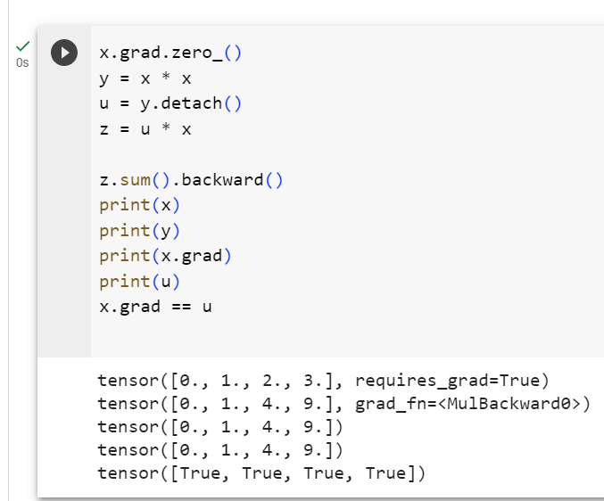
Sometimes, we wish to move some calculations outside of the recorded computational graph. For example, say that we use the input to create some auxiliary intermediate terms for which we do not want to compute a gradient. In this case, we need to detach the respective computational graph from the final result. The following toy example makes this clearer: suppose we have z = x * y and y = x * x but we want to focus on the direct influence of x on z rather than the influence conveyed via y. In this case, we can create a new variable u that takes the same value as y but whose provenance (how it was created) has been wiped out. Thus u has no ancestors in the graph and gradients do not flow through u to x. For example, taking the gradient of z = x * u will yield the result u, (not 3 * x * x as you might have expected since z = x * x * x).

때로는 기록된 계산 그래프 외부로 일부 계산을 이동하고 싶을 때도 있습니다. 예를 들어 입력을 사용하여 기울기를 계산하지 않으려는 일부 보조 중간 항을 생성한다고 가정해 보겠습니다. 이 경우 최종 결과에서 해당 계산 그래프를 분리해야 합니다. 다음  toy 예제는 이를 더 명확하게 해줍니다. z = x * y 및 y = x * x가 있지만 y를 통해 전달되는 영향보다는 x가 z에 미치는 직접적인 영향에 초점을 맞추고 싶다고 가정합니다. 이 경우 y와 동일한 값을 가지지만 출처(생성 방법)가 지워진 새 변수 u를 만들 수 있습니다. 따라서 u에는 그래프에 조상이 없으며 기울기는 u를 통해 x로 흐르지 않습니다. 예를 들어, z = x * u의 기울기를 취하면 결과 u가 생성됩니다(z = x * x * x 이후 예상했던 3 * x * x가 아님).

x.grad.zero_()
y = x * x
u = y.detach()
z = u * x

z.sum().backward()
x.grad == u

이 코드는 PyTorch를 사용하여 그래디언트(미분)와 .detach() 메서드의 역할을 설명하는 예제입니다. 아래에서 코드를 한 줄씩 설명하겠습니다.

x.grad는 x에 대한 그래디언트(미분)를 나타내는 PyTorch 텐서입니다. 이 코드는 이전에 계산된 그래디언트를 지우고 새로운 그래디언트를 계산할 준비를 합니다.

새로운 텐서 y를 생성하며, 이는 x의 제곱을 계산한 결과입니다.

.detach() 메서드는 텐서를 분리(detach)하고 그래디언트 연산을 중단합니다. 이는 u가 y와 동일한 값을 가지지만 그래디언트가 연결되어 있지 않음을 의미합니다.

z는 u와 x의 곱셈으로 계산됩니다.

z의 모든 원소의 합에 대한 그래디언트를 계산합니다. 이러한 그래디언트 계산은 역전파(backpropagation)를 통해 수행됩니다.

• 이 코드는 x.grad와 u를 비교합니다. 여기서 x.grad는 z.sum()에 대한 그래디언트이며, u는 y를 detach하여 생성된 텐서입니다. 이 둘은 같은 값을 가지므로 이 비교는 True를 반환합니다.

즉, x.grad는 z.sum()에 대한 그래디언트이며, 이는 u를 사용하여 x를 곱한 결과인 z에 대한 그래디언트와 같습니다.detach() 메서드를 사용하여 그래디언트 연산을 분리함으로써 그래디언트가 일부 연산에서 중지되도록 할 수 있습니다.

tensor([True, True, True, True])

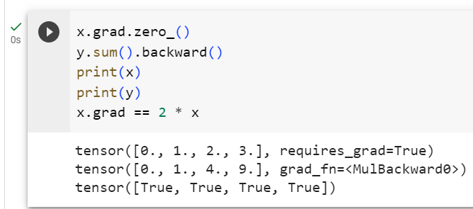
Note that while this procedure detaches y’s ancestors from the graph leading to z, the computational graph leading to y persists and thus we can calculate the gradient of y with respect to x.

이 절차가 z로 이어지는 그래프에서 y의 조상을 분리하는 동안 y로 이어지는 계산 그래프는 지속되므로 x에 대한 y의 기울기를 계산할 수 있습니다.

x.grad.zero_()
y.sum().backward()
x.grad == 2 * x

이 코드는 PyTorch를 사용하여 그래디언트(미분)를 계산하는 예제입니다. 아래에서 코드를 한 줄씩 설명하겠습니다.

x.grad는 x에 대한 그래디언트(미분)를 나타내는 PyTorch 텐서입니다. 이 코드는 이전에 계산된 그래디언트를 지우고 새로운 그래디언트를 계산할 준비를 합니다. zero_() 메서드는 그래디언트를 모두 0으로 초기화합니다.

y의 모든 원소의 합에 대한 그래디언트를 계산합니다. 이러한 그래디언트 계산은 역전파(backpropagation)를 통해 수행됩니다. 여기서 y는 x의 제곱인 텐서입니다.

• 이 코드는 x.grad와 2 * x를 비교합니다. x.grad는 y.sum()에 대한 그래디언트이며, 이것은 y가 x의 제곱이므로 2 * x입니다. 따라서 이 비교는 True를 반환합니다.

즉, x.grad는 y를 x로 미분한 결과이며, 이는 y가 2 * x의 형태를 가지는 관계를 반영합니다. 이것은 연쇄 법칙(Chain Rule)을 통해 계산되며, y가 x에 대한 제곱 함수인 경우 그래디언트는 2 * x가 됩니다.

tensor([True, True, True, True])

2.5.4. Gradients and Python Control Flow

So far we reviewed cases where the path from input to output was well defined via a function such as z = x * x * x. Programming offers us a lot more freedom in how we compute results. For instance, we can make them depend on auxiliary variables or condition choices on intermediate results. One benefit of using automatic differentiation is that even if building the computational graph of a function required passing through a maze of Python control flow (e.g., conditionals, loops, and arbitrary function calls), we can still calculate the gradient of the resulting variable. To illustrate this, consider the following code snippet where the number of iterations of the while loop and the evaluation of the if statement both depend on the value of the input a.

지금까지 우리는 z = x * x * x와 같은 함수를 통해 입력에서 출력까지의 경로가 잘 정의된 사례를 검토했습니다. 프로그래밍은 결과를 계산하는 방법에 있어 훨씬 더 많은 자유를 제공합니다. 예를 들어, 중간 결과에 대한 보조 변수나 조건 선택에 의존하도록 만들 수 있습니다. 자동 미분을 사용하면 미로 같은 Python 제어 흐름(예: 조건문, 루프 및 임의 함수 호출)을 통과해야 하는 함수의 계산 그래프를 작성하더라도 결과 변수의 기울기를 계속 계산할 수 있다는 이점이 있습니다. 이를 설명하기 위해 while 루프의 반복 횟수와 if 문의 평가가 모두 입력 a의 값에 따라 달라지는 다음 코드 조각을 고려해보세요.

def f(a):
    b = a * 2
    while b.norm() < 1000:
        b = b * 2
    if b.sum() > 0:
        c = b
    else:
        c = 100 * b
    return c

이 코드는 파이썬 함수 f(a)를 정의합니다. 이 함수는 입력으로 스칼라 텐서 a를 받아서 다음과 같은 작업을 수행합니다.

1. b라는 새로운 변수를 생성하고 a에 2를 곱한 값을 할당합니다.
2. b의 L2 노름(norm)이 1000보다 작을 때까지 b를 2배씩 계속해서 곱해갑니다. 이것은 b가 L2 노름이 1000보다 커질 때까지 반복하는 루프입니다.
3. 만약 b의 원소들의 합이 0보다 크다면, c에 b를 할당합니다.
4. 그렇지 않다면 (즉, b의 원소들의 합이 0 이하인 경우), c에 100을 곱한 b를 할당합니다.
5. 최종적으로 c를 반환합니다.

이 함수는 입력 a를 사용하여 b를 계산하고, 이후에 b의 크기와 합을 고려하여 c를 정합니다. c의 값은 a와 b에 따라 다르며, 함수의 결과로 반환됩니다.

Below, we call this function, passing in a random value, as input. Since the input is a random variable, we do not know what form the computational graph will take. However, whenever we execute f(a) on a specific input, we realize a specific computational graph and can subsequently run backward.

아래에서는 이 함수를 호출하여 임의의 값을 입력으로 전달합니다. 입력이 랜덤 변수이기 때문에 계산 그래프가 어떤 형태를 취할지 알 수 없습니다. 그러나 특정 입력에 대해 f(a)를 실행할 때마다 특정 계산 그래프를 실현하고 이후에 역방향으로 실행할 수 있습니다.

a = torch.randn(size=(), requires_grad=True)
d = f(a)
d.backward()

이 코드는 PyTorch를 사용하여 작성된 것으로 보이는 예제입니다. 코드는 다음과 같은 작업을 수행합니다:

1. a라는 이름의 스칼라 텐서를 생성합니다. requires_grad=True 매개변수를 사용하여 a에 대한 경사도(gradient)가 계산되도록 설정합니다.
2. 이전에 정의한 f(a) 함수를 호출하여 a를 입력으로 사용하고, 이를 d에 할당합니다.
3. backward 메서드를 사용하여 d의 경사도를 계산합니다. 이것은 연쇄 법칙(chain rule)을 사용하여 d를 a에 대한 함수로 간주하고, d의 a에 대한 경사도를 계산합니다.

즉, 코드는 a에서 f(a)로의 계산 그래프를 구성하고, f(a)의 결과 d에 대한 a의 경사도를 계산합니다. 이렇게 하면 a.grad에 a에 대한 경사도가 저장됩니다.

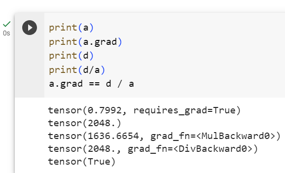
Even though our function f is, for demonstration purposes, a bit contrived, its dependence on the input is quite simple: it is a linear function of a with piecewise defined scale. As such, f(a) / a is a vector of constant entries and, moreover, f(a) / a needs to match the gradient of f(a) with respect to a.

함수 f는 데모 목적으로 약간 인위적으로 만들어졌지만 입력에 대한 의존성은 매우 간단합니다. 부분적으로 정의된 스케일을 사용하는 a의 선형 함수입니다. 따라서 f(a) / a는 상수 항목으로 구성된 벡터이며 더욱이 f(a) / a는 a에 대한 f(a)의 기울기와 일치해야 합니다.

a.grad == d / a

이 코드는 a.grad와 d를 a로 나눈 값인 d / a를 비교하여 결과를 확인합니다.

a.grad는 a에 대한 경사도(gradient)를 나타내며, 이 값은 .backward()를 호출하여 계산됩니다.

d는 f(a) 함수의 결과를 나타내는 변수입니다.

따라서, a.grad는 d를 a로 미분한 값이 됩니다. 코드는 이 계산된 경사도 a.grad와 d / a를 비교하여 두 값이 동일한지 확인합니다.

이 비교가 참인 경우, 이는 PyTorch의 자동 미분이 제대로 작동하고 있다는 것을 의미합니다. 즉, d를 a로 미분한 결과가 d / a와 일치한다는 것을 의미합니다.

tensor(True)

Dynamic control flow is very common in deep learning. For instance, when processing text, the computational graph depends on the length of the input. In these cases, automatic differentiation becomes vital for statistical modeling since it is impossible to compute the gradient a priori.

동적 제어 흐름은 딥러닝에서 매우 일반적입니다. 예를 들어 텍스트를 처리할 때 계산 그래프는 입력 길이에 따라 달라집니다. 이러한 경우 사전에 기울기를 계산하는 것이 불가능하기 때문에 통계 모델링에 자동 미분이 필수적입니다.

2.5.5. Discussion

You have now gotten a taste of the power of automatic differentiation. The development of libraries for calculating derivatives both automatically and efficiently has been a massive productivity booster for deep learning practitioners, liberating them so they can focus on less menial. Moreover, autograd lets us design massive models for which pen and paper gradient computations would be prohibitively time consuming. Interestingly, while we use autograd to optimize models (in a statistical sense) the optimization of autograd libraries themselves (in a computational sense) is a rich subject of vital interest to framework designers. Here, tools from compilers and graph manipulation are leveraged to compute results in the most expedient and memory-efficient manner.

이제 자동 미분의 힘을 맛보셨습니다. 도함수를 자동으로 효율적으로 계산하기 위한 라이브러리의 개발은 딥 러닝 실무자들의 생산성을 대폭 향상시켜 그들이 덜 천박한 일에 집중할 수 있도록 해방시켜 주었습니다. 게다가, autograd를 사용하면 펜과 종이의 그라디언트 계산에 엄청난 시간이 소요되는 대규모 모델을 설계할 수 있습니다. 흥미롭게도, 우리가 모델을 최적화하기 위해(통계적 의미에서) autograd를 사용하는 반면, autograd 라이브러리 자체의 최적화(계산적 의미에서)는 프레임워크 설계자들에게 매우 중요한 주제입니다. 여기서는 컴파일러 도구와 그래프 조작을 활용하여 가장 편리하고 메모리 효율적인 방식으로 결과를 계산합니다.

For now, try to remember these basics: (i) attach gradients to those variables with respect to which we desire derivatives; (ii) record the computation of the target value; (iii) execute the backpropagation function; and (iv) access the resulting gradient.

지금은 다음 기본 사항을 기억해 보십시오. (i) 도함수를 원하는 변수에 기울기를 적용합니다. (ii) 목표값의 계산을 기록하고; (iii) 역전파 기능을 실행합니다. (iv) 결과 그래디언트에 액세스합니다.

2.5.6. Exercises

https://d2l.ai/chapter_preliminaries/calculus.html

2.4. Calculus

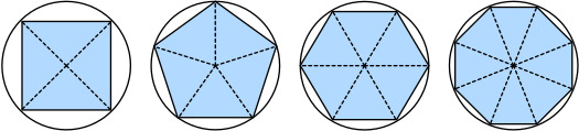
For a long time, how to calculate the area of a circle remained a mystery. Then, in Ancient Greece, the mathematician Archimedes came up with the clever idea to inscribe a series of polygons with increasing numbers of vertices on the inside of a circle (Fig. 2.4.1). For a polygon with n vertices, we obtain n triangles. The height of each triangle approaches the radius r as we partition the circle more finely. At the same time, its base approaches 2 π r/n, since the ratio between arc and secant approaches 1 for a large number of vertices. Thus, the area of the polygon approaches n⋅r⋅1/2(2 π r /n)= π r **2.

오랫동안 원의 넓이를 계산하는 방법은 미스터리로 남아 있었습니다. 그런 다음 고대 그리스의 수학자 아르키메데스는 원 내부에 정점 수가 증가하는 일련의 다각형을 새기는 영리한 아이디어를 생각해 냈습니다(그림 2.4.1). n개의 꼭지점을 가진 다각형의 경우 n개의 삼각형을 얻습니다. 원을 더 세밀하게 분할할수록 각 삼각형의 높이는 반지름 r에 가까워집니다. 동시에, 그 밑변은 2π r/n에 가까워집니다. 왜냐하면 호와 시컨트 사이의 비율이 많은 수의 꼭지점에 대해 1에 가까워지기 때문입니다. 따라서 다각형의 면적은 n⋅r⋅1/2(2 π r /n)= π r **2에 가까워집니다.

This limiting procedure is at the root of both differential calculus and integral calculus. The former can tell us how to increase or decrease a function’s value by manipulating its arguments. This comes in handy for the optimization problems that we face in deep learning, where we repeatedly update our parameters in order to decrease the loss function. Optimization addresses how to fit our models to training data, and calculus is its key prerequisite. However, do not forget that our ultimate goal is to perform well on previously unseen data. That problem is called generalization and will be a key focus of other chapters.

이 제한 절차는 미분 계산 calculus  과 적분 계산 integral calculus 의 기초입니다. 전자는 인수를 조작하여 함수의 값을 늘리거나 줄이는 방법을 알려줄 수 있습니다. 이는 손실 함수를 줄이기 위해 매개변수를 반복적으로 업데이트하는 딥러닝에서 직면하는 최적화 문제에 유용합니다. 최적화는 모델을 훈련 데이터에 맞추는 방법을 다루며, 미적분학은 핵심 전제 조건입니다. 그러나 우리의 궁극적인 목표는 이전에 볼 수 없었던 데이터를 잘 활용하는 것임을 잊지 마십시오. 이 문제를 일반화 generalization  라고 하며 다른 장에서 중점적으로 다룰 것입니다.

%matplotlib inline
import numpy as np
from matplotlib_inline import backend_inline
from d2l import torch as d2l

주어진 코드는 Python 코드로, Jupyter Notebook 또는 IPython 환경에서 사용됩니다. 코드는 다음과 같은 작업을 수행합니다:

1. %matplotlib inline: 이 코드는 Jupyter Notebook에서 사용하는 "매직 명령어" 중 하나로, 그래프나 그림을 출력할 때 그림을 노트북 내부에 표시하도록 설정하는 역할을 합니다. 이렇게 하면 그림이 노트북 내에서 바로 볼 수 있습니다.
2. import numpy as np: NumPy 라이브러리를 불러옵니다. NumPy는 파이썬의 수치 계산과 배열 처리에 유용한 라이브러리로, 주로 다차원 배열과 관련된 작업에 사용됩니다. np는 일반적으로 NumPy의 별칭으로 사용됩니다.
3. from matplotlib_inline import backend_inline: matplotlib_inline 라이브러리에서 backend_inline 모듈을 가져옵니다. 이 모듈은 Matplotlib 그래프를 노트북 내에서 인라인으로 표시할 때 사용됩니다.
4. from d2l import torch as d2l: D2L (Dive into Deep Learning) 라이브러리에서 torch 모듈을 가져온 다음, 이 모듈을 d2l이라는 별칭으로 사용합니다. D2L은 딥러닝 및 머신러닝 교육과 관련된 코드와 자료를 제공하는 라이브러리로, torch 모듈은 PyTorch를 기반으로 한 딥러닝 코드를 작성하기 위해 사용됩니다.

이 코드는 주로 딥러닝 및 머신러닝 관련 작업을 수행하고 시각화를 위한 환경 설정을 위해 사용됩니다. 또한 이 코드는 Jupyter Notebook 또는 IPython 환경에서 노트북 내에서 그래프 및 그림을 표시하기 위한 설정을 제공합니다.

2.4.1. Derivatives and Differentiation

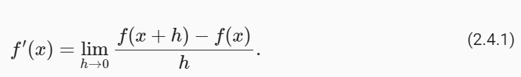
Put simply, a derivative is the rate of change in a function with respect to changes in its arguments. Derivatives can tell us how rapidly a loss function would increase or decrease were we to increase or decrease each parameter by an infinitesimally small amount. Formally, for functions ƒ : ℝ → ℝ , that map from scalars to scalars, the derivative of ƒ  at a point x is defined as

간단히 말해서, 도함수 derivative  는 인수의 변화에 대한 함수의 변화율입니다. Derivatives  은 각 매개변수를 극소량씩 늘리거나 줄이면 손실 함수가 얼마나 빠르게 증가하거나 감소하는지 알려줄 수 있습니다. 공식적으로, 스칼라에서 스칼라로 매핑되는 함수 f : ℝ → ℝ에 대해 점 x에서 의 도함수는 다음과 같이 정의됩니다.

lim (극한) 이란?

In mathematics, "lim" is an abbreviation for the limit. The limit is a fundamental concept in calculus and analysis that describes the behavior of a function or sequence as it approaches a certain value or approaches infinity or negative infinity.

수학에서 "lim"은 "극한(limit)"의 줄임말로 사용됩니다. 극한은 미적분학과 해석학에서 중요한 개념으로, 함수나 수열이 특정한 값을 향하거나 무한대 또는 음의 무한대를 향하는 과정을 기술합니다.

The limit of a function f(x) as x approaches a particular value, say 'a', is denoted as:

특정 값 'a'로 접근할 때 함수 f(x)의 극한은 다음과 같이 나타납니다:

lim (x → a) f(x)

This notation represents the value that the function approaches as x gets closer and closer to 'a'. In other words, it describes what happens to the function as x gets infinitely close to 'a'.

이 표기법은 x가 'a'에 점점 가까워질 때 함수가 어떻게 동작하는지를 설명합니다. 다시 말해, x가 'a'에 무한히 가까워질 때 함수가 어떻게 행동하는지를 나타냅니다.

Limits are used to study the behavior of functions, analyze continuity, and find derivatives and integrals in calculus. They are a crucial tool for understanding the fundamental properties and characteristics of functions, especially in the context of differential and integral calculus. The concept of limits is also essential in real analysis, where it is used to rigorously define continuity, convergence, and other key mathematical concepts.

극한은 미적분학에서 함수의 행동을 연구하고 연속성을 분석하며, 미분 및 적분을 찾는 데 사용되는 중요한 도구입니다. 극한은 함수의 기본적인 특성과 특징을 이해하는 데 필수적이며, 특히 미분 및 적분 미적분학의 맥락에서 중요합니다. 극한의 개념은 또한 해석학에서 사용되어 연속성, 수렴 및 기타 주요 수학적 개념을 엄밀하게 정의하는 데 필수적입니다.

This term on the right hand side is called a limit and it tells us what happens to the value of an expression as a specified variable approaches a particular value. This limit tells us what the ratio between a perturbation ℎ and the change in the function value  f(x+ℎ)−  f(x) converges to as we shrink its size to zero.

오른쪽에 있는 용어는 극한 limit  이라고 하며 지정된 변수가 특정 값에 접근할 때 표현식의 값에 어떤 일이 발생하는지 알려줍니다. 이 극한 limit 는 크기를 0으로 줄이면 섭동 perturbation  ℎ와 함수 값 f(x+ℎ)− f(x)의 변화 사이의 비율이 수렴되는 것을 알려줍니다.

When f ′(x) exists, f  is said to be differentiable at x; and when f ′(x) exists for all x on a set, e.g., the interval [a,b], we say that f  is differentiable on this set. Not all functions are differentiable, including many that we wish to optimize, such as accuracy and the area under the receiving operating characteristic (AUC). However, because computing the derivative of the loss is a crucial step in nearly all algorithms for training deep neural networks, we often optimize a differentiable surrogate instead.

f ′(x)가 존재할 때 f는 x에서 미분 가능하다고 합니다. 그리고 f ′(x)가 세트의 모든 x에 대해 존재할 때(예: 구간 [a,b]), 우리는 f가 이 세트에서 미분 가능하다고 말합니다. 정확도, 수신 작동 특성(AUC) 하의 영역 등 최적화하려는 많은 기능을 포함하여 모든 기능이 차별화 가능한 것은 아닙니다. 그러나 손실의 도함수 derivative  를 계산하는 것은 심층 신경망 훈련을 위한 거의 모든 알고리즘에서 중요한 단계이기 때문에 대신 미분 가능한 대리자를 최적화하는 경우가 많습니다.

We can interpret the derivative f ′(x) as the instantaneous rate of change of f(x) with respect to x. Let’s develop some intuition with an example. Define u= f(x)=3x**2 − 4x.

도함수 f'(x)를 x에 대한 f(x)의 순간 변화율로 해석할 수 있습니다. 예를 들어 직관력을 키워 봅시다. u= f(x)=3x**2−4x를 정의합니다.

def f(x):
    return 3 * x ** 2 - 4 * x

주어진 코드는 파이썬에서 정의한 함수를 설명하고 있습니다. 함수 이름은 f이며, 주어진 입력(x)에 대한 출력을 계산하는 방법을 정의합니다. 함수의 내용은 다음과 같이 나타납니다:

이 코드의 설명은 다음과 같습니다:

1. def f(x):: def 키워드는 파이썬 함수를 정의하기 위해 사용되며, 함수 이름인 f를 정의합니다. 괄호 안에 있는 x는 함수의 입력 매개변수(parameter)입니다. 이 함수는 x라는 입력을 받아서 계산을 수행하고 결과를 반환합니다.
2. return 3 * x ** 2 - 4 * x: 이 줄은 함수의 본문(body)을 정의합니다. 주어진 x를 사용하여 함수가 수행할 계산을 기술합니다. 여기서는 입력 x를 이용하여 다음의 계산을 수행합니다:
   • x를 제곱한 후 3을 곱하고,
   • x를 4 곱한 다음 뺍니다.

이 함수는 주어진 x 값에 대한 결과를 반환합니다. 예를 들어, f(2)를 호출하면 x에 2를 대입하여 3 * 2 ** 2 - 4 * 2를 계산하고, 결과로 -4를 반환할 것입니다.

이 함수를 사용하면 주어진 입력값 x에 대한 함수의 출력을 계산할 수 있으며, 이러한 함수 정의는 미적분 및 수학적 모델링과 같은 다양한 수학적 응용 분야에서 사용됩니다.

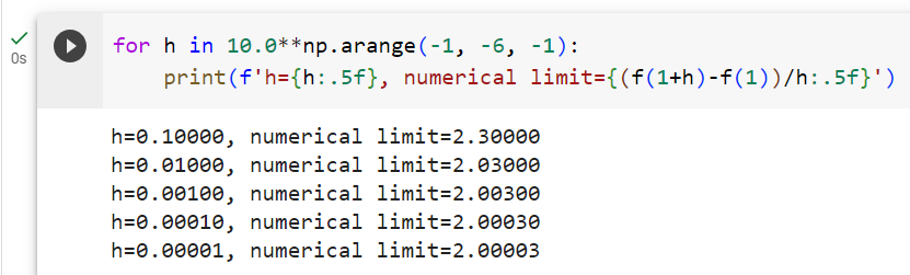
Setting x=1, we see that f(x+ℎ)− f(x)/ℎ approaches 2 as ℎ approaches 0. While this experiment lacks the rigor of a mathematical proof, we can quickly see that indeed f′(1)=2.

x=1로 설정하면 ℎ가 0에 가까워짐에 따라 f(x+ℎ)− f(x)/ℎ도 2에 가까워지는 것을 알 수 있습니다. 이 실험에는 수학적 증명의 엄격함이 부족하지만, 우리는 실제로 'f′(1)=2'라는 것을 빨리 알 수 있습니다.

for h in 10.0**np.arange(-1, -6, -1):
    print(f'h={h:.5f}, numerical limit={(f(1+h)-f(1))/h:.5f}')

주어진 코드는 파이썬의 반복문을 사용하여 함수 f(x)의 수치 미분(numerical derivative)을 계산하고 출력하는 작업을 수행합니다. 코드는 h 값의 범위를 설정하고, 각 h에 대해 f(x) 함수의 미분 값을 계산하고 출력합니다. 아래는 코드의 설명입니다:

1. for h in 10.0**np.arange(-1, -6, -1): 이 줄은 h라는 변수를 사용하여 반복을 설정합니다. np.arange(-1, -6, -1)는 -1에서 -6까지 1씩 감소하는 수열을 생성합니다. 그리고 10.0**를 사용하여 각 수열의 값에 10의 지수를 적용하여 h 값을 생성합니다. 이렇게 함으로써 h는 0.1, 0.01, 0.001, 0.0001, 0.00001의 값을 순서대로 가지게 됩니다.
2. print(f'h={h:.5f}, numerical limit={(f(1+h)-f(1))/h:.5f}'): 이 줄은 각 h 값에 대한 미분 값을 계산하고 출력합니다.
   • h={h:.5f}: h의 값을 소수 다섯 번째 자리까지 출력합니다.
   • numerical limit={(f(1+h)-f(1))/h:.5f}: f(1+h)에서 f(1)을 뺀 다음 h로 나눈 값을 소수 다섯 번째 자리까지 출력합니다. 이 값은 f(x) 함수의 수치 미분을 나타내며, h 값이 작을수록 정확한 미분 값을 얻을 수 있습니다.

따라서 이 코드는 서로 다른 h 값에 대해 f(x) 함수의 수치 미분 값을 계산하고 출력하여, h 값이 작아질수록 정확한 미분 값을 얻는 과정을 보여줍니다. 이러한 과정은 미분 근사를 이해하고 미분 값을 추정하는 데 사용됩니다.

h=0.10000, numerical limit=2.30000
h=0.01000, numerical limit=2.03000
h=0.00100, numerical limit=2.00300
h=0.00010, numerical limit=2.00030
h=0.00001, numerical limit=2.00003

There are several equivalent notational conventions for derivatives. Given y=f(x), the following expressions are equivalent:

derivatives 에 대한 몇 가지 동등한 표기 규칙이 있습니다. y=f(x)라고 가정하면 다음 표현식은 동일합니다.

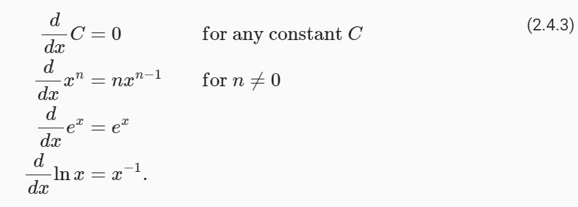
where the symbols d/dx and D are differentiation operators. Below, we present the derivatives of some common functions:

여기서 기호 d/dx와 D는 미분 연산자 differentiation operators 입니다. 아래에서는 몇 가지 일반적인 함수의   derivatives 을 제시합니다.

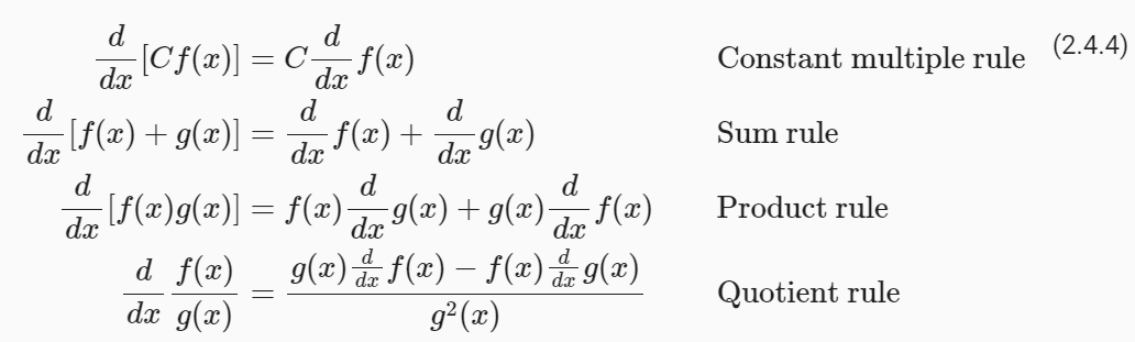
Functions composed from differentiable functions are often themselves differentiable. The following rules come in handy for working with compositions of any differentiable functions f and g, and constant C.

미분 가능한 함수로 구성된 함수는 종종 그 자체로 미분 가능합니다. 다음 규칙은 미분 가능한 함수 f와 g 및 상수 C의 구성 작업에 유용합니다.

Using this, we can apply the rules to find the derivative of 3x**2 − 4x via

이를 사용하여 다음을 통해 3x**2 − 4x의 도함수를 찾는 규칙을 적용할 수 있습니다.

Plugging in x=1 shows that, indeed, the derivative equals 2 at this location. Note that derivatives tell us the slope of a function at a particular location.

x=1을 대입하면 실제로 이 위치에서 도함수는 2와 같다는 것을 알 수 있습니다. 도함수 derivatives  는 특정 위치에서 함수의 기울기를 알려줍니다.

2.4.2. Visualization Utilities

We can visualize the slopes of functions using the matplotlib library. We need to define a few functions. As its name indicates, use_svg_display tells matplotlib to output graphics in SVG format for crisper images. The comment #@save is a special modifier that allows us to save any function, class, or other code block to the d2l package so that we can invoke it later without repeating the code, e.g., via d2l.use_svg_display().

matplotlib 라이브러리를 사용하여 함수의 기울기를 시각화할 수 있습니다. 몇 가지 함수를 정의해야 합니다. 이름에서 알 수 있듯이 use_svg_display는 matplotlib에게 보다 선명한 이미지를 위해 SVG 형식으로 그래픽을 출력하도록 지시합니다. #@save 주석은 함수, 클래스 또는 기타 코드 블록을 d2l 패키지에 저장하여 나중에 코드를 반복하지 않고(예: d2l.use_svg_display()를 통해) 호출할 수 있도록 하는 특수 수정자 special modifier 입니다.

def use_svg_display():  #@save
    """Use the svg format to display a plot in Jupyter."""
    backend_inline.set_matplotlib_formats('svg')

주어진 코드는 Jupyter Notebook 환경에서 그래프나 그림을 SVG(Scalable Vector Graphics) 형식으로 표시하는 함수를 정의하는 파이썬 코드입니다. 아래는 코드의 설명입니다:

1. def use_svg_display():: 이 코드는 use_svg_display라는 이름의 함수를 정의합니다. 이 함수는 그래프나 그림을 SVG 형식으로 표시하도록 설정하는 역할을 합니다.
2. backend_inline.set_matplotlib_formats('svg'): 이 함수 내에서는 backend_inline 라이브러리의 set_matplotlib_formats 함수를 호출합니다. 이 함수는 Matplotlib 그래프의 출력 형식을 설정하는 역할을 합니다. 여기서 'svg'를 사용하여 SVG 형식으로 그래프를 설정합니다. SVG 형식은 확대하더라도 이미지가 깨지지 않고 고품질로 표시되며, Jupyter Notebook 환경에서 렌더링할 때 특히 유용합니다.

따라서 이 코드는 Jupyter Notebook 환경에서 그래프를 그릴 때 그래프의 형식을 SVG로 설정하여, 그래프가 화면에 고해상도로 표시되도록 하는 함수를 정의하고 있습니다. 이 함수를 사용하면 Jupyter Notebook에서 품질 좋은 그래프를 생성하고 시각화할 때 유용합니다.

Conveniently, we can set figure sizes with set_figsize. Since the import statement from matplotlib import pyplot as plt was marked via #@save in the d2l package, we can call d2l.plt.

편리하게도 set_figsize를 사용하여 그림 크기를 설정할 수 있습니다. matplotlib import pyplot as plt의 import 문이 d2l 패키지의 #@save를 통해 표시되었으므로 d2l.plt를 호출할 수 있습니다.

def set_figsize(figsize=(3.5, 2.5)):  #@save
    """Set the figure size for matplotlib."""
    use_svg_display()
    d2l.plt.rcParams['figure.figsize'] = figsize

주어진 코드는 Matplotlib를 사용하여 그림의 크기를 설정하는 함수를 정의하는 파이썬 코드입니다. 아래는 코드의 설명입니다:

1. def set_figsize(figsize=(3.5, 2.5)):: 이 코드는 set_figsize라는 이름의 함수를 정의합니다. 이 함수는 그림의 크기를 설정하는 역할을 합니다. figsize 매개변수를 사용하여 원하는 그림 크기를 지정할 수 있으며, 기본값은 (3.5, 2.5)로 설정되어 있습니다.
2. use_svg_display(): use_svg_display 함수를 호출하여 그래프를 SVG 형식으로 표시하도록 설정합니다. 이전 질문에 설명한 대로, SVG 형식은 고품질 그래프를 표시하는 데 유용합니다.
3. d2l.plt.rcParams['figure.figsize'] = figsize: Matplotlib의 rcParams를 사용하여 그림의 크기를 설정합니다. figsize 매개변수에 지정된 크기로 그림을 설정합니다. 이것은 Matplotlib 그래프의 기본 크기를 변경하는 것으로, figsize를 통해 그림의 가로와 세로 크기를 지정할 수 있습니다.

따라서 이 코드는 Matplotlib를 사용하여 그림의 크기를 설정하는 함수를 정의하고 있으며, 그림 크기를 사용자 지정하거나 기본 설정을 변경하는 데 사용됩니다. 이를 통해 생성되는 그림은 원하는 크기로 표시되며, 시각화 결과를 조절할 수 있습니다.

The set_axes function can associate axes with properties, including labels, ranges, and scales.

set_axes 함수는 축을 레이블, 범위, 스케일 등의 속성과 연결할 수 있습니다.

#@save
def set_axes(axes, xlabel, ylabel, xlim, ylim, xscale, yscale, legend):
    """Set the axes for matplotlib."""
    axes.set_xlabel(xlabel), axes.set_ylabel(ylabel)
    axes.set_xscale(xscale), axes.set_yscale(yscale)
    axes.set_xlim(xlim),     axes.set_ylim(ylim)
    if legend:
        axes.legend(legend)
    axes.grid()

주어진 코드는 Matplotlib 그래프의 축(axis) 설정을 수행하는 함수를 설명하는 파이썬 코드입니다. 이 함수를 사용하면 그래프의 축 레이블, 범위, 스케일, 범례, 그리드 등을 설정할 수 있습니다. 아래는 코드의 설명입니다:

1. def set_axes(axes, xlabel, ylabel, xlim, ylim, xscale, yscale, legend):: 이 코드는 set_axes라는 이름의 함수를 정의합니다. 이 함수는 Matplotlib 그래프의 축 설정을 담당합니다. 함수는 다음과 같은 매개변수를 사용합니다:
   • axes: 설정할 축(axis) 객체.
   • xlabel: x-축 레이블.
   • ylabel: y-축 레이블.
   • xlim: x-축 범위.
   • ylim: y-축 범위.
   • xscale: x-축 스케일.
   • yscale: y-축 스케일.
   • legend: 범례 설정.
2. axes.set_xlabel(xlabel), axes.set_ylabel(ylabel): x-축과 y-축의 레이블을 설정합니다.
3. axes.set_xscale(xscale), axes.set_yscale(yscale): x-축과 y-축의 스케일을 설정합니다. 스케일은 "linear" 또는 "log"와 같은 값으로 설정할 수 있으며, 스케일을 변경하면 축의 데이터 표시 방식이 변경됩니다.
4. axes.set_xlim(xlim), axes.set_ylim(ylim): x-축과 y-축의 범위를 설정합니다. 범위는 그래프에서 보여질 데이터의 최솟값과 최댓값을 지정합니다.
5. if legend: axes.legend(legend): 만약 legend 매개변수가 주어지면 그래프에 범례를 추가합니다. 범례는 그래프에서 각 선 또는 데이터 시리즈를 설명하는 레이블을 표시하는 데 사용됩니다.
6. axes.grid(): 그리드를 추가하여 그래프에 격자 눈금을 표시합니다. 격자 눈금은 데이터의 위치를 더 쉽게 파악할 수 있도록 도와줍니다.

이 함수를 사용하면 Matplotlib 그래프의 축을 사용자 정의하고, 그래프를 보다 명확하게 표시하는 데 도움이 됩니다.

With these three functions, we can define a plot function to overlay multiple curves. Much of the code here is just ensuring that the sizes and shapes of inputs match.

이 세 가지 함수를 사용하면 여러 곡선을 오버레이하는 플롯 함수를 정의할 수 있습니다. 여기 코드의 대부분은 입력의 크기와 모양이 일치하는지 확인하는 것입니다.

#@save
def plot(X, Y=None, xlabel=None, ylabel=None, legend=[], xlim=None,
         ylim=None, xscale='linear', yscale='linear',
         fmts=('-', 'm--', 'g-.', 'r:'), figsize=(3.5, 2.5), axes=None):
    """Plot data points."""

    def has_one_axis(X):  # True if X (tensor or list) has 1 axis
        return (hasattr(X, "ndim") and X.ndim == 1 or isinstance(X, list)
                and not hasattr(X[0], "__len__"))

    if has_one_axis(X): X = [X]
    if Y is None:
        X, Y = [[]] * len(X), X
    elif has_one_axis(Y):
        Y = [Y]
    if len(X) != len(Y):
        X = X * len(Y)

    set_figsize(figsize)
    if axes is None:
        axes = d2l.plt.gca()
    axes.cla()
    for x, y, fmt in zip(X, Y, fmts):
        axes.plot(x,y,fmt) if len(x) else axes.plot(y,fmt)
    set_axes(axes, xlabel, ylabel, xlim, ylim, xscale, yscale, legend)

주어진 코드는 데이터 포인트를 그리는 함수를 설명하는 파이썬 코드입니다. 이 함수를 사용하면 데이터 포인트를 그래프로 표시할 수 있으며, 그래프의 모양, 축, 범위, 스케일, 범례, 그리드 등을 설정할 수 있습니다. 아래는 코드의 설명입니다:

1. plot(X, Y=None, xlabel=None, ylabel=None, legend=[], xlim=None, ylim=None, xscale='linear', yscale='linear', fmts=('-', 'm--', 'g-.', 'r:'), figsize=(3.5, 2.5), axes=None): 이 함수는 데이터 포인트를 그리는 함수로, 다양한 설정 옵션을 제공합니다. 이 함수는 다음과 같은 매개변수를 사용합니다:
   • X: x-축에 대한 데이터 포인트 또는 데이터 포인트 리스트.
   • Y: y-축에 대한 데이터 포인트 또는 데이터 포인트 리스트. 기본값은 None이며, 이 경우 X가 y-축 데이터로 사용됩니다.
   • xlabel: x-축 레이블.
   • ylabel: y-축 레이블.
   • legend: 범례 설정. 여러 데이터 시리즈에 대한 범례를 지정할 수 있습니다.
   • xlim: x-축 범위 설정.
   • ylim: y-축 범위 설정.
   • xscale: x-축 스케일 설정. 기본값은 "linear"로 설정되어 있습니다.
   • yscale: y-축 스케일 설정. 기본값은 "linear"로 설정되어 있습니다.
   • fmts: 그래프의 스타일 설정. 여러 다른 선 스타일을 제공하며, 기본값은 ('-', 'm--', 'g-.', 'r:')로 설정되어 있습니다.
   • figsize: 그래프의 크기 설정. 기본값은 (3.5, 2.5)로 설정되어 있습니다.
   • axes: 그래프를 그릴 Matplotlib 축 객체. 기본값은 None으로 설정되어 있으며, 필요한 경우 사용자가 직접 설정할 수 있습니다.
2. def has_one_axis(X): 이 내부 함수는 주어진 데이터(X)가 1차원 배열 또는 리스트인지 확인합니다. 1차원이면 True를 반환하고, 그렇지 않으면 False를 반환합니다.
3. if has_one_axis(X): X = [X]: 만약 X가 1차원 배열이라면, X를 원소가 하나인 리스트로 변환합니다. 이렇게 함으로써 여러 데이터 시리즈를 다룰 때 편리하게 처리할 수 있습니다.
4. if Y is None: X, Y = [[]] * len(X), X: 만약 Y가 주어지지 않았다면, X를 y-축 데이터로 사용하기 위해 Y를 X로 설정합니다. 그리고 X를 원소가 비어 있는 리스트로 설정합니다.
5. set_figsize(figsize): 그래프의 크기를 figsize에 지정된 크기로 설정하는 함수를 호출합니다.
6. if axes is None: axes = d2l.plt.gca(): 만약 축(axes)가 주어지지 않았다면, 현재 활성화된 Matplotlib 축 객체를 가져와서 사용합니다.
7. axes.cla(): 축 객체를 초기화하여 이전에 그려진 그래프를 지우고 새로운 그래프를 그릴 준비를 합니다.
8. for x, y, fmt in zip(X, Y, fmts): axes.plot(x, y, fmt) if len(x) else axes.plot(y, fmt): X와 Y에 대한 데이터 시리즈와 스타일(fmt)을 순회하면서 그래프를 그립니다. 만약 x 데이터 시리즈가 비어 있다면(len(x) == 0), y 데이터 시리즈를 그래프로 그립니다.
9. set_axes(axes, xlabel, ylabel, xlim, ylim, xscale, yscale, legend): set_axes 함수를 호출하여 축의 레이블, 범위, 스케일, 범례, 그리드 등을 설정합니다.

이 함수를 사용하면 주어진 데이터 포인트를 그래프로 시각화하고, 그래프의 모양과 설정을 유연하게 조절할 수 있습니다. 이는 데이터 시각화 및 그래프 생성에 유용한 도구입니다.

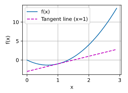
Now we can plot the function u=f(x) and its tangent line y=2x−3 at x=1, where the coefficient 2 is the slope of the tangent line.

이제 x=1에서 함수 u=f(x)와 접선 y=2x−3을 그릴 수 있습니다. 여기서 계수 2는 접선의 기울기입니다.

x = np.arange(0, 3, 0.1)
plot(x, [f(x), 2 * x - 3], 'x', 'f(x)', legend=['f(x)', 'Tangent line (x=1)'])

주어진 코드는 주어진 범위에서 함수 f(x)와 x=1에서의 접선을 그래프로 표시하는 예제 코드입니다. 아래는 코드의 설명입니다:

1. x = np.arange(0, 3, 0.1): 이 코드는 0에서 3까지의 범위에서 0.1 간격으로 숫자를 생성하여 x에 할당합니다. 이렇게 생성된 x 값은 함수 f(x)와 접선을 그래프로 그릴 때 x-축 값으로 사용됩니다.
2. plot(x, [f(x), 2 * x - 3], 'x', 'f(x)', legend=['f(x)', 'Tangent line (x=1)']): plot 함수를 호출하여 그래프를 그립니다. 이때, 다음 매개변수들이 사용됩니다:
   • x: x-축 데이터로 사용될 범위(0에서 3까지의 값).
   • [f(x), 2 * x - 3]: y-축 데이터로 사용될 값. 여기서 f(x)는 함수 f(x)의 값이고, 2 * x - 3은 x=1에서의 접선의 방정식입니다.
   • 'x': x-축 레이블로 사용될 문자열.
   • 'f(x)': y-축 레이블로 사용될 문자열.
   • legend=['f(x)', 'Tangent line (x=1)']: 범례 설정으로, 각 데이터 시리즈에 대한 설명을 제공합니다.

이 코드는 x 범위에서 f(x) 함수와 x=1에서의 접선을 그래프로 그립니다. 이를 통해 함수와 해당 지점에서의 기울기를 시각화할 수 있습니다.

2.4.3. Partial Derivatives and Gradients

Thus far, we have been differentiating functions of just one variable. In deep learning, we also need to work with functions of many variables. We briefly introduce notions of the derivative that apply to such multivariate functions.

지금까지 우리는 단 하나의 변수에 대한 함수를 차별화해 왔습니다. 딥러닝에서는 다양한 변수의 함수를 다루어야 합니다. 우리는 그러한 다변량 함수에 적용되는 미분의 개념을 간략하게 소개합니다.

Let y=f(x1,x2,…,xn) be a function with n variables. The partial derivative of y with respect to its i th parameter xi is

y=f(x1,x2,…,xn)을 n개의 변수를 갖는 함수로 둡니다. i 번째 매개변수 xi에 대한 y의 편도함수 multivariate functions는 다음과 같습니다.

To calculate ∂y/ ∂xi, we can treat x1,…,xi−1,xi+1,…,xn as constants and calculate the derivative of y with respect to xi. The following notational conventions for partial derivatives are all common and all mean the same thing:

∂y/ ∂xi를 계산하려면 x1,…,xi−1,xi+1,…,xn을 상수로 처리하고 xi에 대한 y의 도함수를 계산할 수 있습니다. 부분 도함수에 대한 다음 표기 규칙은 모두 공통적이며 모두 같은 의미입니다.

We can concatenate partial derivatives of a multivariate function with respect to all its variables to obtain a vector that is called the gradient of the function. Suppose that the input of function f: ℝ**n→ ℝ  is an n-dimensional vector x=[x1,x2,…,xn]**⊤ and the output is a scalar. The gradient of the function f with respect to x is a vector of n partial derivatives:

모든 변수에 대해 다변량 함수의 부분 도함수를 연결하여 함수의 기울기라고 하는 벡터를 얻을 수 있습니다. 함수 f: ℝ**n→ ℝ의 입력이 n차원 벡터 x=[x1,x2,…,xn]**⊤이고 출력이 스칼라라고 가정합니다. x에 대한 함수 f의 기울기는 n 편도함수의 벡터입니다.

When there is no ambiguity, ∇_xf(x) is typically replaced by ∇f(x). The following rules come in handy for differentiating multivariate functions:

모호성 ambiguity 이 없으면 ∇_xf(x)는 일반적으로 ∇f(x)로 대체됩니다. 다변량 함수를 차별화하는 데 다음 규칙이 유용합니다.

Similarly, for any matrix X, we have ∇_x|X|²_F=2X.

마찬가지로, 임의의 행렬 X에 대해 ∇_x|X|²_F=2X가 됩니다.

2.4.4. Chain Rule

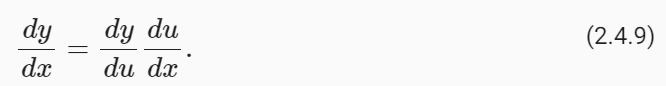
In deep learning, the gradients of concern are often difficult to calculate because we are working with deeply nested functions (of functions (of functions…)). Fortunately, the chain rule takes care of this. Returning to functions of a single variable, suppose that y=f(g(x)) and that the underlying functions y=f(u) and u=g(x) are both differentiable. The chain rule states that

딥 러닝에서는 깊게 중첩된 함수(함수 중(함수…))로 작업하기 때문에 관심 기울기를 계산하기 어려운 경우가 많습니다. 다행히도 체인 규칙이 이를 처리합니다. 단일 변수의 함수로 돌아가서, y=f(g(x))와 기본 함수 y=f(u) 및 u=g(x)가 모두 미분 가능하다고 가정합니다. 체인 규칙은 다음과 같이 명시합니다.

Turning back to multivariate functions, suppose that y=f(u) has variables u1,u2,…,un, where each ui=gi(X) has variables x1,x2,…,xn, i.e., u=g(x). Then the chain rule states that

다변량 함수로 돌아가서, y=f(u)에 변수 u1,u2,…,un이 있다고 가정합니다. 여기서 각 ui=gi(X)에는 변수 x1,x2,…,xn이 있습니다. 즉, u=g(x) . 그런 다음 체인 규칙은 다음과 같이 명시합니다.

where A∈ ℝ ^n×m is a matrix that contains the derivative of vector u with respect to vector x. Thus, evaluating the gradient requires computing a vector–matrix product. This is one of the key reasons why linear algebra is such an integral building block in building deep learning systems.

여기서 A∈ ℝ^n×m은 벡터 x에 대한 벡터 u의 도함수를 포함하는 행렬입니다. 따라서 기울기를 평가하려면 벡터-행렬 곱을 계산해야 합니다. 이것이 선형 대수학이 딥 러닝 시스템을 구축하는 데 필수적인 구성 요소인 주요 이유 중 하나입니다.

2.4.5. Discussion

While we have just scratched the surface of a deep topic, a number of concepts already come into focus: first, the composition rules for differentiation can be applied routinely, enabling us to compute gradients automatically. This task requires no creativity and thus we can focus our cognitive powers elsewhere. Second, computing the derivatives of vector-valued functions requires us to multiply matrices as we trace the dependency graph of variables from output to input. In particular, this graph is traversed in a forward direction when we evaluate a function and in a backwards direction when we compute gradients. Later chapters will formally introduce backpropagation, a computational procedure for applying the chain rule.

우리는 단지 깊은 주제의 표면만 긁었을 뿐이지만 이미 여러 가지 개념에 초점을 맞추고 있습니다. 첫째, 미분을 위한 합성 규칙을 일상적으로 적용하여 기울기를 자동으로 계산할 수 있습니다. 이 작업에는 창의성이 필요하지 않으므로 인지 능력을 다른 곳에 집중할 수 있습니다. 둘째, 벡터 값 함수의 도함수를 계산하려면 출력에서 입력까지 변수의 종속성 그래프를 추적하면서 행렬을 곱해야 합니다. 특히, 이 그래프는 함수를 평가할 때 정방향으로 이동하고 기울기를 계산할 때 역방향으로 이동합니다. 이후 장에서는 체인 규칙을 적용하기 위한 계산 절차인 역전파를 공식적으로 소개할 것입니다.

From the viewpoint of optimization, gradients allow us to determine how to move the parameters of a model in order to lower the loss, and each step of the optimization algorithms used throughout this book will require calculating the gradient.

최적화 관점에서 기울기를 사용하면 손실을 낮추기 위해 모델의 매개변수를 이동하는 방법을 결정할 수 있으며, 이 책 전체에서 사용되는 최적화 알고리즘의 각 단계에서는 기울기 계산이 필요합니다.

2.4.6. Exercises

https://d2l.ai/chapter_preliminaries/linear-algebra.html

2.3. Linear Algebra

By now, we can load datasets into tensors and manipulate these tensors with basic mathematical operations. To start building sophisticated models, we will also need a few tools from linear algebra. This section offers a gentle introduction to the most essential concepts, starting from scalar arithmetic and ramping up to matrix multiplication.

이제 데이터 세트를 텐서에 로드하고 기본적인 수학 연산을 통해 이러한 텐서를 조작할 수 있습니다. 정교한 모델 구축을 시작하려면 선형 대수학의 몇 가지 도구도 필요합니다. 이 섹션에서는 스칼라 산술부터 시작하여 행렬 곱셈까지 가장 필수적인 개념을 부드럽게 소개합니다.

import torch

1. import torch: 이 코드는 PyTorch 라이브러리를 현재 Python 스크립트 또는 환경으로 가져옵니다. PyTorch는 딥러닝 및 텐서 연산을 위한 라이브러리로, 다양한 딥러닝 모델을 구축하고 학습시키며 텐서 관련 작업을 수행하는 데 사용됩니다.

2.3.1. Scalars

Most everyday mathematics consists of manipulating numbers one at a time. Formally, we call these values scalars. For example, the temperature in Palo Alto is a balmy 72 degrees Fahrenheit. If you wanted to convert the temperature to Celsius you would evaluate the expression c=5/9( ƒ −32), setting ƒ  to 72. In this equation, the values 5, 9, and 32 are constant scalars. The variables c and ƒ  in general represent unknown scalars.

대부분의 일상 수학은 한 번에 하나씩 숫자를 조작하는 것으로 구성됩니다. 공식적으로는 이러한 값을 스칼라라고 부릅니다. 예를 들어, 팔로알토(Palo Alto)의 기온은 화씨 72도입니다. 온도를 섭씨로 변환하려면 c=5/9( f −32) 표현식을 평가하고 f를 72로 설정합니다. 이 방정식에서 값 5, 9, 32는 상수 스칼라입니다. 변수 c와 f는 일반적으로 알 수 없는 스칼라를 나타냅니다.

We denote scalars by ordinary lower-cased letters (e.g., x, y, and z) and the space of all (continuous) real-valued scalars by ℝ . For expedience, we will skip past rigorous definitions of spaces: just remember that the expression x∈ ℝ  is a formal way to say that x is a real-valued scalar. The symbol ∈ (pronounced “in”) denotes membership in a set. For example, x,y∈{0,1} indicates that x and y are variables that can only take values 0 or 1.

스칼라는 일반 소문자(예: x, y, z)로 표시하고 모든(연속) 실수 값 스칼라의 공간은 ℝ로 표시합니다. 편의상 공간에 대한 엄격한 정의는 생략하겠습니다. x∈ ℝ라는 표현은 x가 실수 값 스칼라임을 나타내는 형식적인 방법이라는 점만 기억하세요. 기호 ∈(“in”으로 발음)는 집합에 속한다는 것을 나타냅니다. 예를 들어, x,y∈{0,1}은 x와 y가 0 또는 1 값만 가질 수 있는 변수임을 나타냅니다.

Scalars are implemented as tensors that contain only one element. Below, we assign two scalars and perform the familiar addition, multiplication, division, and exponentiation operations.

스칼라는 하나의 요소만 포함하는 텐서로 구현됩니다. 아래에서는 두 개의 스칼라를 할당하고 익숙한 덧셈, 곱셈, 나눗셈 및 지수 연산을 수행합니다.

x = torch.tensor(3.0)
y = torch.tensor(2.0)

x + y, x * y, x / y, x**y, x-y

주어진 코드는 PyTorch를 사용하여 두 개의 텐서 x와 y를 생성하고, 이를 활용하여 다양한 수학 연산을 수행하는 예제입니다. 아래는 코드의 설명입니다:

1. x = torch.tensor(3.0): x라는 이름의 PyTorch 텐서를 생성하고, 값으로 3.0을 할당합니다.
2. y = torch.tensor(2.0): y라는 이름의 PyTorch 텐서를 생성하고, 값으로 2.0을 할당합니다.
3. x + y: x와 y의 덧셈을 수행합니다. 결과로 새로운 텐서가 생성되며, 이 텐서의 값은 3.0 + 2.0으로 5.0이 됩니다.
4. x * y: x와 y의 곱셈을 수행합니다. 결과로 새로운 텐서가 생성되며, 이 텐서의 값은 3.0 * 2.0으로 6.0이 됩니다.
5. x / y: x를 y로 나눗셈을 수행합니다. 결과로 새로운 텐서가 생성되며, 이 텐서의 값은 3.0 / 2.0으로 1.5가 됩니다.
6. x**y: x를 y 제곱 연산을 수행합니다. 결과로 새로운 텐서가 생성되며, 이 텐서의 값은 3.0의 2.0 제곱으로 9.0이 됩니다.
7. x - y: x와 y의 뺄셈을 수행합니다. 결과로 새로운 텐서가 생성되며, 이 텐서의 값은 3.0 - 2.0으로 1.0이 됩니다.

코드를 실행하면 각 연산의 결과가 출력됩니다. PyTorch를 사용하면 텐서를 활용하여 다양한 수학적 연산을 수행할 수 있으며, 딥러닝 모델의 학습과 예측 등에 활용됩니다.

(tensor(5.), tensor(6.), tensor(1.5000), tensor(9.), tensor(1.))

2.3.2. Vectors

For current purposes, you can think of a vector as a fixed-length array of scalars. As with their code counterparts, we call these scalars the elements of the vector (synonyms include entries and components). When vectors represent examples from real-world datasets, their values hold some real-world significance. For example, if we were training a model to predict the risk of a loan defaulting, we might associate each applicant with a vector whose components correspond to quantities like their income, length of employment, or number of previous defaults. If we were studying the risk of heart attack, each vector might represent a patient and its components might correspond to their most recent vital signs, cholesterol levels, minutes of exercise per day, etc. We denote vectors by bold lowercase letters, (e.g., x, y, and z).

현재 목적상 벡터를 스칼라의 고정 길이 배열로 생각할 수 있습니다. 해당 코드와 마찬가지로 이러한 스칼라를 벡터의 요소라고 부릅니다(동의어에는 항목과 구성 요소가 포함됨). 벡터가 실제 데이터 세트의 예를 나타내는 경우 해당 값은 실제 의미를 갖습니다. 예를 들어, 대출 불이행 위험을 예측하기 위해 모델을 훈련하는 경우 각 지원자를 소득, 고용 기간 또는 이전 불이행 횟수와 같은 수량에 해당하는 구성요소가 있는 벡터와 연결할 수 있습니다. 심장 마비의 위험을 연구하는 경우 각 벡터는 환자를 나타낼 수 있으며 그 구성 요소는 가장 최근의 활력 징후, 콜레스테롤 수치, 일일 운동 시간(분) 등에 해당할 수 있습니다. 벡터는 굵은 소문자로 표시됩니다(예: x, y, z).

Vectors are implemented as 1 st-order tensors. In general, such tensors can have arbitrary lengths, subject to memory limitations. Caution: in Python, as in most programming languages, vector indices start at 0, also known as zero-based indexing, whereas in linear algebra subscripts begin at 1 (one-based indexing).

벡터는 1차 텐서로 구현됩니다. 일반적으로 이러한 텐서는 메모리 제한에 따라 임의의 길이를 가질 수 있습니다. 주의: Python에서는 대부분의 프로그래밍 언어와 마찬가지로 벡터 인덱스가 0부터 시작합니다(0부터 시작하는 인덱싱이라고도 함). 반면 선형 대수학 첨자는 1(1부터 시작하는 인덱싱)에서 시작합니다.

x = torch.arange(3)
x

주어진 코드는 PyTorch를 사용하여 텐서 x를 생성하는 예제입니다. 아래는 코드의 설명입니다:

1. x = torch.arange(3): torch.arange() 함수를 사용하여 x라는 이름의 PyTorch 텐서를 생성합니다. torch.arange() 함수는 주어진 범위 내의 정수를 순서대로 생성하는 함수로, 여기서는 0부터 2까지의 정수를 생성하게 됩니다. 따라서 x는 [0, 1, 2]라는 값을 가지는 1차원 텐서가 됩니다.
2. x: 텐서 x를 출력합니다. 이 코드는 텐서 x의 내용을 화면에 출력하여 확인할 수 있습니다.

결과적으로, 코드를 실행하면 x라는 이름의 PyTorch 텐서가 생성되며, 그 값은 [0, 1, 2]인 1차원 배열로 출력됩니다. PyTorch의 텐서는 수학 및 딥러닝 연산에 사용되며, 다양한 데이터 처리 및 모델 학습 작업에 활용됩니다.

tensor([0, 1, 2])

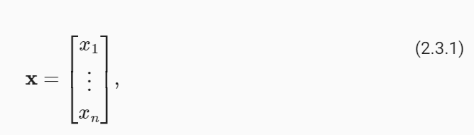
We can refer to an element of a vector by using a subscript. For example, x₂ denotes the second element of x. Since x₂ is a scalar, we do not bold it. By default, we visualize vectors by stacking their elements vertically.

아래 첨자를 사용하여 벡터의 요소를 참조할 수 있습니다. 예를 들어 x₂는 x의 두 번째 요소를 나타냅니다. x₂는 스칼라이므로 굵게 표시하지 않습니다. 기본적으로 벡터의 요소를 수직으로 쌓아서 벡터를 시각화합니다.

Here x₁,…,x_n are elements of the vector. Later on, we will distinguish between such column vectors and row vectors whose elements are stacked horizontally. Recall that we access a tensor’s elements via indexing.

여기서 x₁,…,x_n은 벡터의 요소입니다. 나중에 이러한 열 벡터와 요소가 가로로 쌓인 행 벡터를 구분할 것입니다. 인덱싱을 통해 텐서의 요소에 액세스한다는 점을 기억하세요.

x[2]

주어진 코드는 PyTorch 텐서 x에서 특정 인덱스에 해당하는 값을 추출하는 예제입니다. 아래는 코드의 설명입니다:

1. x[2]: 이 코드는 PyTorch 텐서 x에서 인덱스 2에 해당하는 값을 추출하는 작업을 수행합니다. 텐서 x는 0부터 시작하는 인덱스를 가지며, 2번 인덱스는 세 번째 원소를 나타냅니다.

예를 들어, 만약 x가 [0, 1, 2]라는 값을 가진 1차원 텐서라면, x[2]는 2번 인덱스에 해당하는 값인 2를 반환합니다.

이 코드를 실행하면 x 텐서에서 해당 인덱스의 값을 추출하여 반환합니다. 결과적으로, x[2]는 x 텐서의 세 번째 원소에 해당하는 값을 반환합니다.

tensor(2)

To indicate that a vector contains n elements, we write x∈ ℝⁿ. Formally, we call n the dimensionality of the vector. In code, this corresponds to the tensor’s length, accessible via Python’s built-in len function.

벡터에 n개의 요소가 포함되어 있음을 나타내기 위해 x∈ ℝⁿ이라고 씁니다. 공식적으로 n을 벡터의 차원이라고 부릅니다. 코드에서 이는 Python의 내장 len 함수를 통해 액세스할 수 있는 텐서의 길이에 해당합니다.

len(x)

주어진 코드는 PyTorch 텐서 x의 길이(원소의 개수)를 반환하는 예제입니다. 아래는 코드의 설명입니다:

1. len(x): 이 코드는 PyTorch 텐서 x의 길이를 반환합니다. 텐서의 길이는 해당 텐서에 포함된 원소의 개수를 나타냅니다.

예를 들어, x가 [0, 1, 2]라는 값을 가진 1차원 텐서라면, len(x)는 3을 반환합니다. 즉, 이 텐서에는 3개의 원소가 포함되어 있습니다.

이 코드를 실행하면 x 텐서의 길이가 반환됩니다. 결과적으로, len(x)는 x 텐서에 포함된 원소의 개수를 나타내는 정수를 반환합니다.

3

We can also access the length via the shape attribute. The shape is a tuple that indicates a tensor’s length along each axis. Tensors with just one axis have shapes with just one element.

Shape 속성을 통해 길이에 접근할 수도 있습니다. 모양은 각 축을 따라 텐서의 길이를 나타내는 튜플입니다. 축이 하나뿐인 텐서는 요소가 하나만 있는 모양을 갖습니다.

x.shape

주어진 코드는 PyTorch 텐서 x의 모양(shape)을 반환하는 예제입니다. 아래는 코드의 설명입니다:

1. x.shape: 이 코드는 PyTorch 텐서 x의 모양(shape)을 반환합니다. 모양은 텐서가 어떻게 구성되어 있는지를 나타내며, 차원과 각 차원의 크기를 포함합니다.

예를 들어, 만약 x가 2차원 텐서이고 모양이 (3, 4)라면, x.shape는 (3, 4)를 반환합니다. 이는 3개의 행과 4개의 열로 이루어진 2차원 텐서임을 나타냅니다.

이 코드를 실행하면 x 텐서의 모양이 반환됩니다. 결과적으로, x.shape는 텐서의 차원과 각 차원의 크기를 나타내는 튜플을 반환합니다.

torch.Size([3])

Oftentimes, the word “dimension” gets overloaded to mean both the number of axes and the length along a particular axis. To avoid this confusion, we use order to refer to the number of axes and dimensionality exclusively to refer to the number of components.

종종 " dimension 차원"이라는 단어는 축 수와 특정 축의 길이를 모두 의미하는 것으로 오버로드됩니다. 이러한 혼란을 피하기 위해 우리는 축 수를 참조하기 위해 순서 order 를 사용하고 구성 요소 수를 참조하기 위해 차원 dimensionality 을 독점적으로 사용합니다.

2.3.3. Matrices

Just as scalars are 0 th-order tensors and vectors are 1 st-order tensors, matrices are 2 nd-order tensors. We denote matrices by bold capital letters (e.g., X, Y, and Z), and represent them in code by tensors with two axes. The expression A∈ ℝ ^m×n indicates that a matrix A contains m×n real-valued scalars, arranged as m rows and n columns. When m=n, we say that a matrix is square. Visually, we can illustrate any matrix as a table. To refer to an individual element, we subscript both the row and column indices, e.g., a_ij is the value that belongs to A’s i th row and j th column:

스칼라가 0차 텐서이고 벡터가 1차 텐서인 것처럼 행렬은 2차 텐서입니다. 행렬은 굵은 대문자(예: X, Y, Z)로 표시하고 두 개의 축이 있는 텐서로 코드로 표시합니다. A∈ ℝ^m×n 표현식은 행렬 A가 m행과 n열로 배열된 m×n 실수 값 스칼라를 포함함을 나타냅니다. m=n일 때, 행렬은 square 이라고 말합니다. 시각적으로 모든 행렬을 테이블로 설명할 수 있습니다. 개별 요소를 참조하기 위해 행과 열 인덱스를 모두 첨자로 표시합니다. 예를 들어 a_ij는 A의 i 번째 행과 j 번째 열에 속하는 값입니다.

In code, we represent a matrix A∈ ℝ m×n  by a 2nd-order tensor with shape (m, n). We can convert any appropriately sized m×n tensor into an m×n matrix by passing the desired shape to reshape:

코드에서는 행렬 A∈ ℝ^m×n을 모양이 (m, n)인 2차 텐서로 표현합니다. 원하는 모양을 전달하여 적절한 크기의 m×n 텐서를 m×n 행렬로 변환할 수 있습니다.

A = torch.arange(6).reshape(3, 2)
A

주어진 코드는 PyTorch를 사용하여 텐서 A를 생성하고, 그 모양을 변경하는 작업을 수행하는 예제입니다. 아래는 코드의 설명입니다:

1. A = torch.arange(6): torch.arange() 함수를 사용하여 0부터 5까지의 정수로 이루어진 1차원 텐서 A를 생성합니다. 이 텐서는 [0, 1, 2, 3, 4, 5]와 같은 값을 가지게 됩니다.
2. .reshape(3, 2): 생성한 텐서 A의 모양을 변경합니다. .reshape() 메서드를 사용하여 텐서의 모양을 변경할 수 있으며, 여기서는 (3, 2) 모양으로 변경합니다. 따라서 텐서 A는 3개의 행과 2개의 열로 이루어진 2차원 텐서가 됩니다.
3. A: 변경된 텐서 A를 출력합니다. 이 코드는 변경된 모양의 텐서 A를 확인할 수 있도록 출력합니다.

결과적으로, 코드를 실행하면 0부터 5까지의 값을 가진 1차원 텐서 A가 생성되고, 그 후 (3, 2) 모양으로 변경된 텐서 A가 출력됩니다. 이처럼 PyTorch를 사용하면 텐서의 모양을 변경하여 데이터를 원하는 형태로 조작할 수 있습니다.

tensor([[0, 1],
        [2, 3],
        [4, 5]])

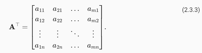
Sometimes we want to flip the axes. When we exchange a matrix’s rows and columns, the result is called its transpose. Formally, we signify a matrix A’s transpose by A^⊤ and if B=A^⊤, then b_ij=a_ji for all i and j. Thus, the transpose of an m×n matrix is an n×m matrix:

때로는 축을 뒤집고 싶을 때도 있습니다. 행렬의 행과 열을 교환할 때의 결과를 전치 transpose 라고 합니다. 공식적으로, 행렬 A의 전치를 A^⊤로 표시하고 B=A^⊤이면 모든 i와 j에 대해 b_ij=a_ji입니다. 따라서 m×n 행렬의 전치는 n×m 행렬입니다.

In code, we can access any matrix’s transpose as follows:

코드에서는 다음과 같이 모든 행렬의 전치에 액세스할 수 있습니다.

A.T

tensor([[0, 2, 4],
        [1, 3, 5]])

주어진 코드 A.T는 PyTorch 텐서 A의 전치(transpose)를 반환하는 작업을 나타냅니다. 아래는 코드의 설명입니다:

1. A.T: 이 코드는 텐서 A의 전치(transpose)를 반환합니다. 전치란 원본 행렬 또는 텐서의 행과 열을 바꾼 것을 의미합니다. 즉, 텐서 A의 행은 열로, 열은 행으로 바뀝니다.

예를 들어, 만약 텐서 A가 다음과 같다면:

A = torch.tensor([[0, 1],
                  [2, 3],
                  [4, 5]])

A.T는 다음과 같이 전치된 텐서를 반환합니다:

tensor([[0, 2, 4],
        [1, 3, 5]])

결과적으로, A.T 코드를 실행하면 텐서 A의 전치된 형태인 새로운 텐서가 반환됩니다. 이렇게 하면 원본 텐서의 행과 열이 바뀐 모양의 텐서를 얻을 수 있습니다.

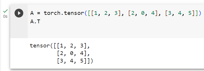
Symmetric matrices are the subset of square matrices that are equal to their own transposes: A=A^⊤. The following matrix is symmetric:

대칭 행렬은 자체 전치와 동일한 정사각형 행렬의 하위 집합입니다(A=A^⊤). 다음 행렬은 대칭입니다.

A = torch.tensor([[1, 2, 3], [2, 0, 4], [3, 4, 5]])
A == A.T

주어진 코드는 PyTorch 텐서 A와 그 전치(A.T) 간의 요소별 비교를 수행하고 결과를 반환하는 예제입니다. 아래는 코드의 설명입니다:

1. A = torch.tensor([[1, 2, 3], [2, 0, 4], [3, 4, 5]]): 텐서 A를 생성합니다. 이 텐서는 3x3 크기의 2차원 배열을 나타내며, 각 요소의 값은 주어진 값으로 초기화됩니다.
2. A.T: 텐서 A의 전치(transpose)를 계산합니다. 이렇게 하면 원본 텐서의 행과 열이 바뀐 형태의 텐서가 생성됩니다.
3. A == A.T: 원본 텐서 A와 그 전치 텐서 A.T 간의 요소별(원소별) 비교를 수행합니다. 두 텐서의 같은 위치에 있는 요소끼리 비교하며, 결과는 두 텐서가 동일한 요소를 가지면 True로, 다른 경우에는 False로 나타납니다.

결과적으로, A == A.T 코드를 실행하면 A와 A의 전치 텐서 A.T 간의 요소별 비교 결과를 반환합니다. 이 코드의 결과는 A와 A.T가 대칭 행렬인 경우에만 모든 요소가 True가 됩니다. 다시 말해, A가 대칭 행렬이라면 A == A.T는 모든 요소가 True를 반환할 것입니다.

tensor([[True, True, True],
        [True, True, True],
        [True, True, True]])

Matrices are useful for representing datasets. Typically, rows correspond to individual records and columns correspond to distinct attributes.

행렬은 데이터 세트를 나타내는 데 유용합니다. 일반적으로 행은 개별 레코드에 해당하고 열은 고유한 속성에 해당합니다.

2.3.4. Tensors

While you can go far in your machine learning journey with only scalars, vectors, and matrices, eventually you may need to work with higher-order tensors. Tensors give us a generic way of describing extensions to nth-order arrays. We call software objects of the tensor class “tensors” precisely because they too can have arbitrary numbers of axes. While it may be confusing to use the word tensor for both the mathematical object and its realization in code, our meaning should usually be clear from context. We denote general tensors by capital letters with a special font face (e.g., X, Y, and Z) and their indexing mechanism (e.g., x_ijk and [X]_1,2i−1,3) follows naturally from that of matrices.

스칼라, 벡터 및 행렬만으로 기계 학습 여정을 멀리할 수 있지만 결국에는 고차 텐서를 사용하여 작업해야 할 수도 있습니다. 텐서는 n차 배열에 대한 확장을 설명하는 일반적인 방법을 제공합니다. 우리는 텐서 클래스의 소프트웨어 객체를 "텐서"라고 부릅니다. 왜냐하면 그들 역시 임의의 수의 축을 가질 수 있기 때문입니다. 수학적 객체와 코드에서의 구현 모두에 대해 텐서라는 단어를 사용하는 것이 혼란스러울 수 있지만 일반적으로 의미는 문맥에서 명확해야 합니다. 일반 텐서를 특수 글꼴(예: X, Y, Z)이 있는 대문자로 표시하며 해당 인덱싱 메커니즘(예: x_ijk 및 [X]_1,2i−1,3)은 자연스럽게 행렬의 인덱싱 메커니즘을 따릅니다.

Tensors will become more important when we start working with images. Each image arrives as a 3rd-order tensor with axes corresponding to the height, width, and channel. At each spatial location, the intensities of each color (red, green, and blue) are stacked along the channel. Furthermore, a collection of images is represented in code by a 4th-order tensor, where distinct images are indexed along the first axis. Higher-order tensors are constructed, as were vectors and matrices, by growing the number of shape components.

이미지 작업을 시작하면 Tensor가 더욱 중요해집니다. 각 이미지는 높이, 너비 및 채널에 해당하는 축이 있는 3차 텐서로 도착합니다. 각 공간 위치에서 각 색상(빨간색, 녹색, 파란색)의 강도가 채널을 따라 누적됩니다. 또한, 이미지 모음은 코드에서 4차 텐서로 표현되며, 여기서 개별 이미지는 첫 번째 축을 따라 인덱싱됩니다. 고차 텐서는 벡터 및 행렬과 마찬가지로 모양 구성 요소의 수를 늘려 구성됩니다.

torch.arange(24).reshape(2, 3, 4)

주어진 코드는 PyTorch를 사용하여 2x3x4 크기의 3차원 텐서를 생성하는 작업을 나타냅니다. 아래는 코드의 설명입니다:

1. torch.arange(24): 이 코드는 0부터 23까지의 정수를 포함하는 1차원 텐서를 생성합니다. torch.arange() 함수는 주어진 범위 내의 정수를 생성하는 함수입니다.
2. .reshape(2, 3, 4): 앞서 생성한 1차원 텐서를 2x3x4 크기의 다차원 텐서로 형태를 변경합니다. .reshape() 메서드를 사용하여 텐서의 모양을 변경할 수 있으며, 여기서는 (2, 3, 4) 모양으로 변경합니다. 따라서 이제 텐서는 3차원 배열로 표현되며, 크기는 2개의 "깊이" (depth), 각 깊이당 3개의 "행" (rows), 그리고 각 행당 4개의 "열" (columns)로 구성됩니다.

결과적으로, torch.arange(24).reshape(2, 3, 4) 코드를 실행하면 2x3x4 크기의 3차원 텐서가 생성됩니다. 이 텐서는 다양한 데이터를 저장하거나 다차원 배열 연산을 수행하는 데 사용될 수 있습니다.

tensor([[[ 0,  1,  2,  3],
         [ 4,  5,  6,  7],
         [ 8,  9, 10, 11]],

        [[12, 13, 14, 15],
         [16, 17, 18, 19],
         [20, 21, 22, 23]]])

2.3.5. Basic Properties of Tensor Arithmetic

Scalars, vectors, matrices, and higher-order tensors all have some handy properties. For example, elementwise operations produce outputs that have the same shape as their operands.

스칼라, 벡터, 행렬 및 고차 텐서는 모두 몇 가지 편리한 속성을 가지고 있습니다. 예를 들어 요소별 연산은 피연산자와 모양이 동일한 출력을 생성합니다.

A = torch.arange(6, dtype=torch.float32).reshape(2, 3)
B = A.clone()  # Assign a copy of A to B by allocating new memory
A, A + B

(tensor([[0., 1., 2.],
         [3., 4., 5.]]),
 tensor([[ 0.,  2.,  4.],
         [ 6.,  8., 10.]]))

주어진 코드는 PyTorch를 사용하여 두 개의 텐서 A와 B를 생성하고, 이를 활용하여 텐서 간의 덧셈 연산을 수행하는 작업을 나타냅니다. 아래는 코드의 설명입니다:

1. A = torch.arange(6, dtype=torch.float32).reshape(2, 3): 먼저, 텐서 A를 생성합니다. torch.arange() 함수는 0부터 시작하여 5까지의 값을 가지는 1차원 텐서를 생성하고, 이를 .reshape(2, 3) 메서드를 사용하여 2x3 크기의 2차원 텐서로 형태를 변경합니다. 결과적으로 A는 다음과 같이 표현됩니다:

tensor([[0., 1., 2.],
        [3., 4., 5.]])

1. B = A.clone(): 다음으로, 텐서 B를 생성합니다. 여기서 A.clone()을 사용하여 텐서 A의 복사본을 만듭니다. 이 때, 새로운 메모리를 할당하여 A와 동일한 값을 가지는 B를 생성합니다. 이로써 A와 B는 동일한 값을 가지지만 서로 다른 메모리 공간을 사용하게 됩니다.
2. A, A + B: 텐서 A와 텐서 B를 출력합니다. 그리고 A + B를 사용하여 두 텐서의 요소별 덧셈 연산을 수행한 결과를 출력합니다. 덧셈 연산은 같은 위치에 있는 요소끼리 더해지며, 결과는 다음과 같이 표시됩니다:

(tensor([[0., 1., 2.],
         [3., 4., 5.]]),
 tensor([[ 0.,  2.,  4.],
         [ 6.,  8., 10.]]))

결과적으로, 코드를 실행하면 두 개의 텐서 A와 B가 생성되고, 이를 사용하여 요소별 덧셈 연산이 수행되어 두 개의 텐서가 반환됩니다. 이렇게 PyTorch를 사용하면 텐서 연산을 쉽게 수행하고, 복사본을 만들어 원본 데이터를 보존할 수 있습니다.

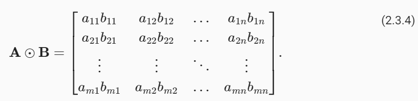
The elementwise product of two matrices is called their Hadamard product (denoted ⊙). We can spell out the entries of the Hadamard product of two matrices A,B∈ ℝ ^m×n:

두 행렬의 요소별 곱을 하다마드 곱(Hadamard product)이라고 합니다(기호 ⊙). 두 행렬 A,B∈ ℝ ^m×n의 Hadamard 곱의 항목을 spell out 할 수 있습니다.

A * B

tensor([[ 0.,  1.,  4.],
        [ 9., 16., 25.]])

주어진 코드 A * B는 PyTorch 텐서 A와 B 간의 요소별 곱셈 연산을 나타냅니다. 아래는 코드의 설명입니다:

1. A * B: 이 코드는 텐서 A와 B 간의 요소별 곱셈을 수행합니다. 요소별 곱셈은 두 텐서의 같은 위치에 있는 요소끼리 곱셈을 수행하며, 결과는 새로운 텐서로 반환됩니다.

예를 들어, A와 B가 다음과 같다면:

A = torch.tensor([[0., 1., 2.],
                  [3., 4., 5.]])
B = torch.tensor([[1., 2., 3.],
                  [4., 5., 6.]])

A * B는 다음과 같이 요소별로 곱셈이 수행된 결과를 반환합니다:

tensor([[ 0.,  2.,  6.],
        [12., 20., 30.]])

결과적으로, A * B 코드를 실행하면 두 개의 텐서 A와 B 간의 요소별 곱셈 연산이 수행되어 새로운 텐서가 반환됩니다. 이렇게 하면 각 요소가 서로 곱해진 결과가 나타납니다. PyTorch를 사용하면 다양한 요소별 연산을 쉽게 수행할 수 있으며, 이를 활용하여 수학적 계산을 수행할 수 있습니다.

Hadamard product (Hadamard 곱)이란?

The Hadamard product, also known as the element-wise product or entrywise product, is a mathematical operation that involves multiplying each corresponding element of two matrices or vectors together.

Hadamard 곱(또는 요소별 곱셈 또는 항별 곱셈)은 두 행렬 또는 벡터의 각 해당 요소를 서로 곱하는 수학적 연산입니다.

Specifically, for two matrices A and B of the same shape (i.e., they have the same number of rows and columns), the Hadamard product C is calculated as follows:

구체적으로, 동일한 모양을 가진 두 행렬 A와 B에 대해 Hadamard 곱 C는 다음과 같이 계산됩니다:

C[i][j] = A[i][j] * B[i][j] for all valid indices i and j.

In other words, each element in the resulting matrix C is obtained by multiplying the corresponding elements of A and B. The Hadamard product differs from the more conventional matrix multiplication (dot product) in which you perform element-wise multiplication and then sum the results.

다시 말해, 결과 행렬 C의 각 요소는 A와 B의 해당 요소를 곱하여 얻어집니다. Hadamard 곱은 요소별 곱셈을 수행하고 결과를 합산하는 일반적인 행렬 곱셈과는 다릅니다.

The Hadamard product is often denoted by a circle with a dot inside it (∘) or by simply using the multiplication symbol (*), without any special operation notation.

Hadamard 곱은 두 행렬 또는 벡터의 각 요소를 독립적으로 처리하려는 경우 요소 간의 관계를 보존하면서 수행할 때 특히 유용합니다. Hadamard 곱은 일반적으로 점(∘)이 내부에 있는 원으로 표시되거나 간단히 곱셈 기호(*)를 사용하여 나타납니다.

The Hadamard product is used in various mathematical and scientific contexts, including linear algebra, signal processing, and statistics. It's particularly useful in cases where you want to perform operations on individual components of matrices or vectors independently, preserving their element-wise relationships.

Hadamard 곱은 선형 대수, 신호 처리 및 통계를 포함한 다양한 수학적 및 과학적 맥락에서 사용됩니다. 이 연산은 행렬이나 벡터의 개별 구성 요소에 대한 연산을 독립적으로 수행하고 요소 간의 관계를 보존할 때 특히 유용합니다.

Adding or multiplying a scalar and a tensor produces a result with the same shape as the original tensor. Here, each element of the tensor is added to (or multiplied by) the scalar.

스칼라와 텐서를 더하거나 곱하면 원래 텐서와 모양이 같은 결과가 생성됩니다. 여기서 텐서의 각 요소는 스칼라에 추가되거나 곱해집니다.

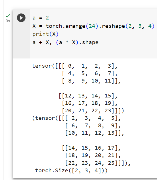
a = 2
X = torch.arange(24).reshape(2, 3, 4)
a + X, (a * X).shape

(tensor([[[ 2,  3,  4,  5],
          [ 6,  7,  8,  9],
          [10, 11, 12, 13]],

         [[14, 15, 16, 17],
          [18, 19, 20, 21],
          [22, 23, 24, 25]]]),
 torch.Size([2, 3, 4]))

주어진 코드는 PyTorch를 사용하여 스칼라 값 a와 3차원 텐서 X 간의 덧셈 연산과 곱셈 연산을 수행하는 작업을 나타냅니다. 아래는 코드의 설명입니다:

1. a = 2: 변수 a에 숫자 2를 할당합니다. 이 값은 스칼라(하나의 숫자)를 나타냅니다.
2. X = torch.arange(24).reshape(2, 3, 4): 0부터 23까지의 정수로 이루어진 1차원 텐서를 생성한 후, .reshape(2, 3, 4) 메서드를 사용하여 이를 2x3x4 크기의 3차원 텐서로 형태를 변경합니다. 결과적으로 X는 3차원 배열로 표현되며, 크기는 2개의 "깊이" (depth), 각 깊이당 3개의 "행" (rows), 그리고 각 행당 4개의 "열" (columns)로 구성됩니다.
3. a + X: 스칼라 값 a와 3차원 텐서 X 간의 요소별 덧셈 연산을 수행합니다. 스칼라 값 a가 X의 각 요소에 더해지며, 결과는 X와 동일한 크기의 텐서로 반환됩니다.
4. (a * X).shape: 스칼라 값 a와 3차원 텐서 X 간의 요소별 곱셈 연산을 수행합니다. 결과로 나오는 텐서의 모양(shape)을 확인합니다. .shape 속성은 텐서의 모양을 반환합니다.

결과적으로, 코드를 실행하면 두 개의 결과가 반환됩니다:

• 첫 번째 결과는 a가 X의 각 요소에 더해져서 생성된 텐서입니다. 이 텐서는 X와 동일한 크기를 가지며, 각 요소는 a와 X의 해당 위치 요소를 더한 값입니다.
• 두 번째 결과는 a가 X의 각 요소에 곱해진 결과인 텐서의 모양(shape)입니다. 이 경우, 곱셈 연산은 모양(shape)을 변경하지 않으므로 (2, 3, 4)와 같은 모양을 가진 원래 X와 동일한 모양을 반환합니다.

이 코드를 통해 PyTorch에서 스칼라와 텐서 간의 연산을 어떻게 수행하는지를 이해할 수 있습니다.

2.3.6. Reduction

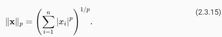
Often, we wish to calculate the sum of a tensor’s elements. To express the sum of the elements in a vector x of length n, we write ∑ⁿ _i=1 x_i. There is a simple function for it:

종종 우리는 텐서 요소의 합을 계산하고 싶습니다. 길이 n의 벡터 x에 있는 요소의 합을 표현하기 위해 ∑ⁿ _i=1 x_i라고 씁니다. 이를 위한 간단한 기능이 있습니다:

x = torch.arange(3, dtype=torch.float32)
x, x.sum()

주어진 코드는 PyTorch를 사용하여 1차원 텐서 x를 생성하고, 그 텐서의 합계를 계산하는 작업을 나타냅니다. 아래는 코드의 설명입니다:

1. x = torch.arange(3, dtype=torch.float32): torch.arange() 함수를 사용하여 0부터 2까지의 정수로 이루어진 1차원 텐서 x를 생성합니다. dtype=torch.float32를 사용하여 텐서의 데이터 타입을 부동소수점(float32)으로 설정합니다.
2. x: 생성한 텐서 x를 출력합니다. 이 코드는 텐서 x를 확인하기 위해 화면에 출력합니다.
3. x.sum(): 텐서 x의 합계를 계산합니다. .sum() 메서드는 텐서의 모든 요소의 합을 반환합니다. 여기서는 x의 요소가 [0.0, 1.0, 2.0]이므로 합계는 0.0 + 1.0 + 2.0으로 3.0이 됩니다.

결과적으로, 코드를 실행하면 텐서 x가 생성되고, 이 텐서의 내용이 출력됩니다. 또한 x.sum()을 호출하여 텐서 x의 합계가 계산되고 출력됩니다. 이 코드는 PyTorch를 사용하여 텐서를 생성하고 기본적인 연산을 수행하는 예제를 보여줍니다.

(tensor([0., 1., 2.]), tensor(3.))

To express sums over the elements of tensors of arbitrary shape, we simply sum over all its axes. For example, the sum of the elements of an m×n matrix A could be written ∑^m _i=1∑ⁿ _j=1 a_ij.

임의 형태의 텐서 요소에 대한 합을 표현하려면 단순히 모든 축에 대한 합을 구하면 됩니다. 예를 들어, m×n 행렬 A의 요소들의 합은 ∑^m _i=1 ∑ⁿ _j=1 a_ij로 쓸 수 있습니다.

A.shape, A.sum()

(torch.Size([2, 3]), tensor(15.))

주어진 코드는 PyTorch 텐서 A의 모양(shape)과 텐서 내의 모든 요소의 합계를 계산하는 작업을 나타냅니다. 아래는 코드의 설명입니다:

1. A.shape: 텐서 A의 모양(shape)을 확인하는 작업입니다. .shape 속성을 사용하면 텐서의 차원과 각 차원의 크기를 나타내는 튜플이 반환됩니다.
2. A.sum(): 텐서 A의 모든 요소의 합계를 계산하는 작업입니다. .sum() 메서드를 사용하면 텐서 내의 모든 요소를 합한 결과가 반환됩니다.

결과적으로, 코드를 실행하면 두 가지 결과가 반환됩니다:

• 첫 번째 결과는 텐서 A의 모양(shape)을 나타내는 튜플입니다. 이 튜플은 텐서의 차원과 각 차원의 크기를 포함하고 있습니다. 예를 들어, (2, 3, 4)와 같은 튜플은 3차원 텐서이며, 첫 번째 차원은 2, 두 번째 차원은 3, 세 번째 차원은 4의 크기를 가집니다.
• 두 번째 결과는 텐서 A 내의 모든 요소의 합계를 나타내는 값입니다. 이 값은 텐서 내의 모든 요소를 합한 결과이므로, A의 모든 요소를 합친 총합이 됩니다.

이 코드는 텐서의 모양과 요소의 합을 확인하는 데 유용하며, 데이터 분석 및 딥러닝 모델 학습 중에 자주 사용됩니다.

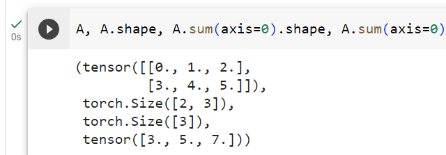
By default, invoking the sum function reduces a tensor along all of its axes, eventually producing a scalar. Our libraries also allow us to specify the axes along which the tensor should be reduced. To sum over all elements along the rows (axis 0), we specify axis=0 in sum. Since the input matrix reduces along axis 0 to generate the output vector, this axis is missing from the shape of the output.

기본적으로 sum 함수를 호출하면 모든 축을 따라 텐서가 줄어들고 결국 스칼라가 생성됩니다. 우리 라이브러리를 사용하면 텐서가 감소되어야 하는 축을 지정할 수도 있습니다. 행(축 0)을 따라 모든 요소를 합산하려면 합산에 axis=0을 지정합니다. 입력 행렬은 출력 벡터를 생성하기 위해 축 0을 따라 감소하므로 이 축은 출력의 모양에서 누락됩니다.

A.shape, A.sum(axis=0).shape

주어진 코드는 PyTorch 텐서 A의 모양(shape)과 axis=0를 사용하여 첫 번째 차원(열)을 따라 합산한 결과의 모양을 확인하는 작업을 나타냅니다. 아래는 코드의 설명입니다:

1. A.shape: 텐서 A의 모양(shape)을 확인하는 작업입니다. .shape 속성을 사용하면 텐서의 차원과 각 차원의 크기를 나타내는 튜플이 반환됩니다.
2. A.sum(axis=0): 텐서 A의 첫 번째 차원(열)을 따라 합산한 결과를 계산합니다. axis 매개변수를 사용하여 어떤 차원을 따라 합산할지 지정할 수 있으며, 여기서는 axis=0을 사용하여 첫 번째 차원을 따라 합산합니다.
3. A.sum(axis=0).shape: 합산된 결과 텐서의 모양(shape)을 확인하는 작업입니다. .shape 속성을 사용하여 모양을 확인합니다.

결과적으로, 코드를 실행하면 두 가지 결과가 반환됩니다:

• 첫 번째 결과는 원래 텐서 A의 모양(shape)을 나타내는 튜플입니다.
• 두 번째 결과는 첫 번째 차원(열)을 따라 합산한 결과 텐서의 모양(shape)을 나타내는 튜플입니다. 이 결과 텐서는 첫 번째 차원이 합산되었기 때문에 원래 텐서보다 한 차원이 줄어듭니다.

이 코드를 통해 PyTorch를 사용하여 텐서의 차원 및 차원 간의 연산을 조작하고 모양(shape)을 확인하는 방법을 이해할 수 있습니다.

(torch.Size([2, 3]), torch.Size([3]))

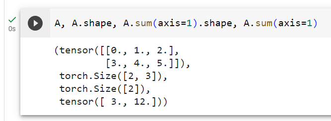
Specifying axis=1 will reduce the column dimension (axis 1) by summing up elements of all the columns.

axis=1을 지정하면 모든 열의 요소를 합산하여 열 차원(축 1)이 줄어듭니다.

A.shape, A.sum(axis=1).shape

주어진 코드는 PyTorch 텐서 A의 모양(shape)과 axis=1을 사용하여 두 번째 차원(행)을 따라 합산한 결과의 모양을 확인하는 작업을 나타냅니다. 아래는 코드의 설명입니다:

1. A.shape: 텐서 A의 모얥(shape)을 확인하는 작업입니다. .shape 속성을 사용하면 텐서의 차원과 각 차원의 크기를 나타내는 튜플이 반환됩니다.
2. A.sum(axis=1): 텐서 A의 두 번째 차원(행)을 따라 합산한 결과를 계산합니다. axis 매개변수를 사용하여 어떤 차원을 따라 합산할지 지정할 수 있으며, 여기서는 axis=1을 사용하여 두 번째 차원을 따라 합산합니다.
3. A.sum(axis=1).shape: 합산된 결과 텐서의 모양(shape)을 확인하는 작업입니다. .shape 속성을 사용하여 모양을 확인합니다.

결과적으로, 코드를 실행하면 두 가지 결과가 반환됩니다:

• 첫 번째 결과는 원래 텐서 A의 모양(shape)을 나타내는 튜플입니다.
• 두 번째 결과는 두 번째 차원(행)을 따라 합산한 결과 텐서의 모양(shape)을 나타내는 튜플입니다. 이 결과 텐서는 두 번째 차원이 합산되었기 때문에 원래 텐서보다 한 차원이 줄어듭니다.

이 코드를 통해 PyTorch를 사용하여 텐서의 차원 및 차원 간의 연산을 조작하고 모양(shape)을 확인하는 방법을 이해할 수 있습니다.

(torch.Size([2, 3]), torch.Size([2]))

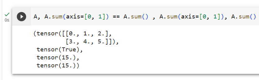
Reducing a matrix along both rows and columns via summation is equivalent to summing up all the elements of the matrix.

합산을 통해 행과 열 모두에서 행렬을 줄이는 것은 행렬의 모든 요소를 합산하는 것과 같습니다.

A.sum(axis=[0, 1]) == A.sum()  # Same as A.sum()

주어진 코드는 PyTorch 텐서 A에 대해 axis=[0, 1]를 사용하여 두 개의 축(차원)을 따라 합산한 결과와 전체 텐서를 합산한 결과를 비교하는 작업을 나타냅니다. 아래는 코드의 설명입니다:

1. A.sum(axis=[0, 1]): 텐서 A에 대해 axis=[0, 1]을 사용하여 0번째 차원(열)과 1번째 차원(행)을 따라 합산한 결과를 계산합니다. 여기서 [0, 1]은 텐서의 0번째 차원과 1번째 차원을 모두 합산하라는 의미입니다. 결과는 전체 텐서의 합계를 나타내게 됩니다.
2. A.sum(): 텐서 A의 모든 요소를 합산한 결과를 계산합니다. .sum() 메서드를 사용하면 텐서 내의 모든 요소를 합산한 결과가 반환됩니다.
3. A.sum(axis=[0, 1]) == A.sum(): A.sum(axis=[0, 1])과 A.sum()의 결과를 비교하는 작업을 수행합니다. 두 결과가 같은지 여부를 확인하기 위한 비교 연산을 수행하며, 결과는 True 또는 False로 나타납니다.

결과적으로, 코드를 실행하면 A.sum(axis=[0, 1])과 A.sum()의 결과를 비교하여 두 값이 동일한지 여부를 확인하는 논리식이 반환됩니다. 이 코드는 텐서의 다차원 연산과 축을 따라 합산하는 방법을 보여주며, axis=[0, 1]을 사용하여 전체 텐서를 합산한 결과와 A.sum()를 사용한 결과가 동일함을 나타냅니다.

tensor(True)

A related quantity is the mean, also called the average. We calculate the mean by dividing the sum by the total number of elements. Because computing the mean is so common, it gets a dedicated library function that works analogously to sum.

관련 수량은 average 이라고도 하는 평균 mean 입니다. 합계를 전체 요소 수로 나누어 평균을 계산합니다. 평균을 계산하는 것은 매우 일반적이기 때문에 합계와 유사하게 작동하는 전용 라이브러리 함수를 얻습니다.

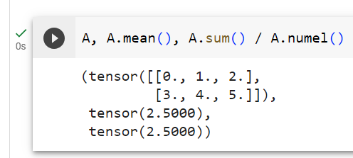
A.mean(), A.sum() / A.numel()

주어진 코드는 PyTorch 텐서 A의 평균과 텐서의 모든 요소의 합계를 요소의 총 개수로 나눈 결과를 계산하는 작업을 나타냅니다. 아래는 코드의 설명입니다:

1. A.mean(): 텐서 A의 평균을 계산합니다. .mean() 메서드를 사용하면 텐서 내의 모든 요소의 평균값이 반환됩니다.
2. A.sum(): 텐서 A의 모든 요소를 합산한 결과를 계산합니다. .sum() 메서드를 사용하면 텐서 내의 모든 요소를 합산한 결과가 반환됩니다.
3. A.numel(): 텐서 A의 요소의 총 개수를 계산합니다. .numel() 메서드는 텐서 내의 모든 요소의 개수를 반환합니다.
4. A.sum() / A.numel(): A.sum()을 텐서의 요소 개수(A.numel())로 나눈 결과를 계산합니다. 이렇게 함으로써 텐서의 평균을 구합니다.

결과적으로, 코드를 실행하면 두 가지 결과가 반환됩니다:

• 첫 번째 결과는 텐서 A의 모든 요소의 평균값을 나타내는 값입니다. 이 값은 텐서의 모든 요소를 더하고 요소의 총 개수로 나눈 결과입니다.
• 두 번째 결과는 텐서 A의 모든 요소를 합산한 값을 나타내는 값입니다.

이 코드를 통해 PyTorch를 사용하여 텐서의 요소를 평균화하고 총합을 계산하는 방법을 이해할 수 있습니다.

(tensor(2.5000), tensor(2.5000))

Likewise, the function for calculating the mean can also reduce a tensor along specific axes.

마찬가지로, 평균을 계산하는 함수는 특정 축을 따라 텐서를 줄일 수도 있습니다.

A.mean(axis=0), A.sum(axis=0) / A.shape[0]

주어진 코드는 PyTorch 텐서 A에 대해 axis=0을 사용하여 0번째 차원(열)을 따라 평균과 합계를 계산한 결과를 비교하는 작업을 나타냅니다. 아래는 코드의 설명입니다:

1. A.mean(axis=0): 텐서 A에 대해 axis=0을 사용하여 0번째 차원(열)을 따라 평균을 계산합니다. axis 매개변수를 사용하여 어떤 차원을 따라 평균을 계산할지 지정할 수 있으며, 여기서는 axis=0을 사용하여 0번째 차원(열)을 따라 평균을 계산합니다.
2. A.sum(axis=0): 텐서 A에 대해 axis=0을 사용하여 0번째 차원(열)을 따라 합계를 계산합니다. axis 매개변수를 사용하여 어떤 차원을 따라 합계를 계산할지 지정할 수 있으며, 여기서는 axis=0을 사용하여 0번째 차원(열)을 따라 합계를 계산합니다.
3. A.shape[0]: 텐서 A의 0번째 차원(열)의 크기를 확인합니다. A.shape은 텐서의 모양(shape)을 나타내는 튜플을 반환하며, 여기서 [0]을 사용하여 튜플의 첫 번째 요소를 얻습니다.
4. A.sum(axis=0) / A.shape[0]: A.sum(axis=0)을 0번째 차원(열)의 크기(A.shape[0])로 나눈 결과를 계산합니다. 이렇게 함으로써 0번째 차원을 따라 합산한 평균을 구합니다.

결과적으로, 코드를 실행하면 두 가지 결과가 반환됩니다:

• 첫 번째 결과는 텐서 A의 0번째 차원(열)을 따라 평균을 계산한 결과입니다.
• 두 번째 결과는 텐서 A의 0번째 차원(열)을 따라 합산한 결과를 텐서의 0번째 차원 크기로 나눈 평균을 나타내는 값입니다.

이 코드를 통해 PyTorch를 사용하여 텐서의 특정 차원을 따라 평균 및 합계를 계산하고, 이를 텐서의 크기로 나누어 평균을 구하는 방법을 이해할 수 있습니다.

(tensor([1.5000, 2.5000, 3.5000]), tensor([1.5000, 2.5000, 3.5000]))

2.3.7. Non-Reduction Sum

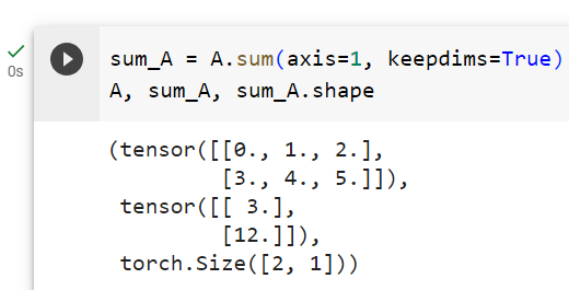
Sometimes it can be useful to keep the number of axes unchanged when invoking the function for calculating the sum or mean. This matters when we want to use the broadcast mechanism.

때로는 합계 또는 평균을 계산하는 함수를 호출할 때 축 수를 변경하지 않고 유지하는 것이 유용할 수 있습니다. 이는 브로드캐스트 메커니즘을 사용하려는 경우 중요합니다.

sum_A = A.sum(axis=1, keepdims=True)
sum_A, sum_A.shape

주어진 코드는 PyTorch 텐서 A에 대해 axis=1을 사용하여 1번째 차원(행)을 따라 합산한 결과를 계산하고, keepdims=True 옵션을 사용하여 결과 텐서의 차원을 유지한 채로 결과를 확인하는 작업을 나타냅니다. 아래는 코드의 설명입니다:

1. A.sum(axis=1, keepdims=True): 텐서 A에 대해 axis=1을 사용하여 1번째 차원(행)을 따라 합산한 결과를 계산합니다. axis 매개변수를 사용하여 어떤 차원을 따라 합산할지 지정할 수 있으며, 여기서는 axis=1을 사용하여 1번째 차원(행)을 따라 합산합니다. keepdims=True 옵션은 결과 텐서의 차원을 유지하도록 설정합니다.
2. sum_A: 합산 결과를 저장하는 변수로 A.sum(axis=1, keepdims=True)의 결과를 할당합니다.
3. sum_A.shape: sum_A 텐서의 모양(shape)을 확인합니다. .shape 속성을 사용하면 텐서의 차원과 각 차원의 크기를 나타내는 튜플을 반환합니다.

결과적으로, 코드를 실행하면 두 가지 결과가 반환됩니다:

• 첫 번째 결과는 텐서 A의 1번째 차원(행)을 따라 합산한 결과를 나타내는 텐서입니다. 이 텐서의 차원은 원래 텐서와 동일한 차원을 가지며, 합산 결과가 유지됩니다.
• 두 번째 결과는 sum_A 텐서의 모양(shape)을 나타내는 튜플입니다.

이 코드를 통해 PyTorch를 사용하여 텐서의 특정 차원을 따라 합산하고, 결과 텐서의 차원을 유지하며 차원의 모양(shape)을 확인하는 방법을 이해할 수 있습니다.

(tensor([[ 3.],
         [12.]]),
 torch.Size([2, 1]))

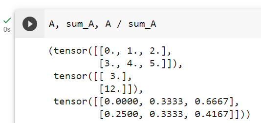
For instance, since sum_A keeps its two axes after summing each row, we can divide A by sum_A with broadcasting to create a matrix where each row sums up to 1.

예를 들어 sum_A는 각 행을 합산한 후 두 개의 축을 유지하므로 브로드캐스팅을 통해 A를 sum_A로 나누어 각 행의 합이 다음과 같은 행렬을 만들 수 있습니다.

A / sum_A

주어진 코드는 PyTorch 텐서 A를 sum_A로 나누는 작업을 나타냅니다. sum_A는 이전 코드에서 A의 1번째 차원(행)을 따라 합산한 결과를 나타내는 텐서입니다. 아래는 코드의 설명입니다:

1. A / sum_A: 텐서 A를 sum_A로 나누는 작업을 수행합니다. 이 작업은 요소별로 (element-wise) 이루어지며, 텐서 A와 sum_A의 같은 위치에 있는 요소끼리 나눗셈을 수행합니다. 결과는 새로운 텐서로 반환됩니다.

결과적으로, 코드를 실행하면 A와 sum_A의 요소별 나눗셈 연산을 수행한 결과인 새로운 텐서가 반환됩니다. 이 코드를 통해 텐서의 요소끼리 나눗셈 연산을 수행하는 방법을 이해할 수 있습니다. 이러한 연산을 사용하면 데이터 정규화나 스케일링과 같은 다양한 작업을 수행할 수 있습니다.

tensor([[0.0000, 0.3333, 0.6667],
        [0.2500, 0.3333, 0.4167]])

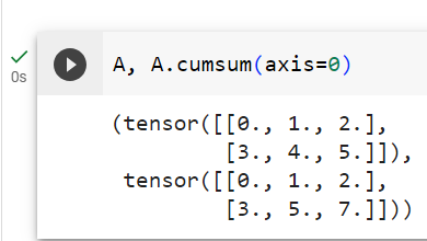
If we want to calculate the cumulative sum of elements of A along some axis, say axis=0 (row by row), we can call the cumsum function. By design, this function does not reduce the input tensor along any axis.

어떤 축(축=0(행 단위))을 따라 A 요소의 누적 합계를 계산하려면 cumsum 함수를 호출할 수 있습니다. 설계상 이 함수는 어떤 축에서도 입력 텐서를 줄이지 않습니다.

A.cumsum(axis=0)

주어진 코드는 PyTorch 텐서 A에 대해 axis=0을 사용하여 0번째 차원(열)을 따라 누적 합계(cumulative sum)를 계산하는 작업을 나타냅니다. 아래는 코드의 설명입니다:

1. A.cumsum(axis=0): 텐서 A에 대해 axis=0을 사용하여 0번째 차원(열)을 따라 누적 합계를 계산합니다. axis 매개변수를 사용하여 어떤 차원을 따라 누적 합계를 계산할지 지정할 수 있으며, 여기서는 axis=0을 사용하여 0번째 차원(열)을 따라 누적 합계를 계산합니다.

결과적으로, 코드를 실행하면 텐서 A의 0번째 차원(열)을 따라 누적 합계를 계산한 결과를 반환합니다. 이 결과 텐서는 원래 텐서와 동일한 모양(shape)을 가지며, 각 요소는 해당 열까지의 누적 합계를 나타냅니다.

이 코드를 통해 PyTorch를 사용하여 텐서의 특정 차원을 따라 누적 합계를 계산하는 방법을 이해할 수 있습니다. 누적 합계는 주어진 차원의 각 위치에서 해당 위치까지의 합계를 나타내는데 사용됩니다.

tensor([[0., 1., 2.],
        [3., 5., 7.]])

2.3.8. Dot Products

So far, we have only performed elementwise operations, sums, and averages. And if this was all we could do, linear algebra would not deserve its own section. Fortunately, this is where things get more interesting. One of the most fundamental operations is the dot product. Given two vectors x,y∈ ℝ ^d, their dot product x^⊤y (also known as inner product, ⟨x,y⟩) is a sum over the products of the elements at the same position: x^⊤y=∑^d _i=1  x_iy_i.

지금까지는 요소별 연산, 합계, 평균만 수행했습니다. 그리고 이것이 우리가 할 수 있는 전부라면 선형 대수학은 그 자체의 섹션을 가질 자격이 없을 것입니다. 다행히도 여기서 상황이 더욱 흥미로워집니다. 가장 기본적인 연산 중 하나는 내적(dot product)입니다. 두 개의 벡터 x,y∈ ℝ^d가 주어지면, 그 내적 x^⊤y(내적이라고도 함, ⟨x,y⟩)는 동일한 위치에 있는 요소의 곱에 대한 합입니다.  x^⊤y=∑^d _i=1  x_iy_i.

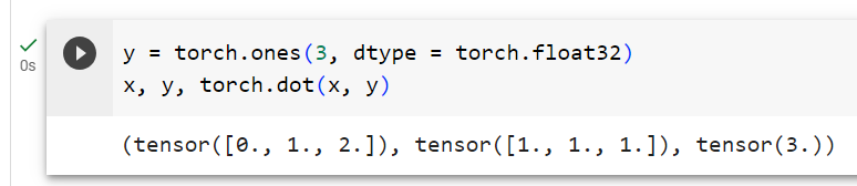
y = torch.ones(3, dtype = torch.float32)
x, y, torch.dot(x, y)

주어진 코드는 PyTorch를 사용하여 두 벡터 x와 y를 생성하고, 이 두 벡터의 내적(dot product)을 계산하는 작업을 나타냅니다. 아래는 코드의 설명입니다:

1. y = torch.ones(3, dtype=torch.float32): 길이가 3인 1차원 텐서 y를 생성합니다. torch.ones() 함수를 사용하여 모든 요소가 1로 초기화된 텐서를 생성하며, dtype 매개변수를 사용하여 데이터 타입을 부동소수점(float32)으로 설정합니다.
2. x: 벡터 x를 생성한 변수입니다. 코드에서 직접 표시되지 않았지만, x는 이전에 어떤 값으로 초기화되었을 것입니다. x는 y와 동일한 길이를 가져야합니다.
3. y: 위에서 생성한 벡터 y입니다.
4. torch.dot(x, y): 벡터 x와 y 사이의 내적(dot product)을 계산합니다. 내적은 두 벡터의 대응하는 요소를 곱한 후 모두 더한 값을 의미합니다. 이 코드는 x와 y 벡터의 내적을 계산하고 결과를 반환합니다.

결과적으로, 코드를 실행하면 x와 y 벡터가 생성되고, 이 두 벡터의 내적이 계산되어 반환됩니다. 내적은 벡터 간의 유사성을 측정하는 데 사용되며, 벡터의 각 성분을 곱한 후 모두 합한 값으로 표현됩니다.

(tensor([0., 1., 2.]), tensor([1., 1., 1.]), tensor(3.))

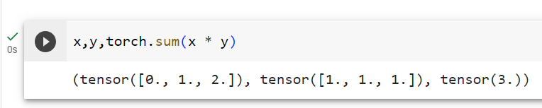
Equivalently, we can calculate the dot product of two vectors by performing an elementwise multiplication followed by a sum:

마찬가지로 요소별 곱셈과 합을 수행하여 두 벡터의 내적을 계산할 수 있습니다.

torch.sum(x * y)

주어진 코드는 PyTorch를 사용하여 두 벡터 x와 y를 요소별로 곱하고 그 결과를 모두 합산하는 작업을 나타냅니다. 코드에서 올바른 방법으로 작성하기 위해서는 torch.sum() 함수를 사용해야 합니다. 아래는 코드의 설명입니다:

1. torch.sum(x * y): 벡터 x와 y의 요소별 곱셈을 수행한 후, 그 결과를 모두 합산합니다. 이 코드는 x와 y의 각 성분을 곱한 후 그 결과를 모두 합산하는 동작을 수행합니다.

결과적으로, 코드를 실행하면 두 벡터 x와 y의 요소별 곱셈 결과가 계산되고, 이 결과를 모두 합산한 값이 반환됩니다. 내적과 유사하지만 내적은 두 벡터의 대응하는 요소를 곱한 후 모두 더하는 것이며, 이 코드는 요소별 곱셈 결과를 모두 더합니다.

tensor(3.)

Dot products are useful in a wide range of contexts. For example, given some set of values, denoted by a vector x∈ ℝⁿ, and a set of weights, denoted by w∈ ℝ ⁿ , the weighted sum of the values in x according to the weights w could be expressed as the dot product x^⊤w. When the weights are nonnegative and sum to 1, i.e., (∑ⁿ_i=1 w_i=1), the dot product expresses a weighted average. After normalizing two vectors to have unit length, the dot products express the cosine of the angle between them. Later in this section, we will formally introduce this notion of length.

내적은 다양한 상황에서 유용합니다. 예를 들어, 벡터 x∈ ℝ ⁿ으로 표시되는 일부 값 세트와 w∈ ℝ ⁿ으로 표시되는 가중치 세트가 주어지면 가중치 w에 따른 x 값의 가중 합은 점으로 표현될 수 있습니다. 제품 x^⊤w. 가중치가 음수가 아니고 합이 1인 경우, 즉 (∑ⁿ _i=1 w_i=1), 내적은 가중 평균을 나타냅니다. 두 벡터를 단위 길이로 정규화한 후, 내적은 두 벡터 사이의 각도의 코사인을 나타냅니다. 이 섹션의 뒷부분에서 길이에 대한 개념을 공식적으로 소개하겠습니다.

2.3.9. Matrix–Vector Products

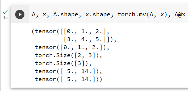
Now that we know how to calculate dot products, we can begin to understand the product between an m×n matrix A and an n-dimensional vector x. To start off, we visualize our matrix in terms of its row vectors where each a^⊤_i∈ ℝⁿ  is a row vector representing the i th row of the matrix A.

이제 내적을 계산하는 방법을 알았으므로 m×n 행렬 A와 n차원 벡터 x 사이의 곱을 이해할 수 있습니다. 시작하려면 각 a^⊤_i∈ ℝⁿ이 행렬 A의 i번째 행을 나타내는 행 벡터인 행 벡터 측면에서 행렬을 시각화합니다.

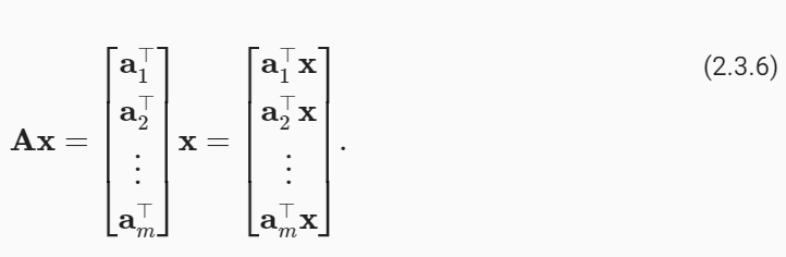
The matrix–vector product Ax is simply a column vector of length m, whose i th element is the dot product a^⊤_i x:

행렬-벡터 곱 Ax는 단순히 길이가 m인 열 벡터이며, i 번째 요소는 내적 a^⊤_i x입니다.

We can think of multiplication with a matrix A∈ ℝ^m×n as a transformation that projects vectors from ℝⁿ to ℝ^m. These transformations are remarkably useful. For example, we can represent rotations as multiplications by certain square matrices. Matrix–vector products also describe the key calculation involved in computing the outputs of each layer in a neural network given the outputs from the previous layer.

행렬 A∈ ℝ ^m×n을 사용한 곱셈을 ℝⁿ에서 ℝ^m으로 벡터를 투영하는 변환으로 생각할 수 있습니다. 이러한 변환은 매우 유용합니다. 예를 들어 회전을 특정 정사각 행렬의 곱셈으로 표현할 수 있습니다. 행렬-벡터 곱은 이전 계층의 출력을 바탕으로 신경망의 각 계층 출력을 계산하는 데 관련된 주요 계산도 설명합니다.

To express a matrix–vector product in code, we use the mv function. Note that the column dimension of A (its length along axis 1) must be the same as the dimension of x (its length). Python has a convenience operator @ that can execute both matrix–vector and matrix–matrix products (depending on its arguments). Thus we can write A@x.

행렬-벡터 곱을 코드로 표현하기 위해 mv 함수를 사용합니다. A의 열 치수(축 1을 따른 길이)는 x의 치수(길이)와 동일해야 합니다. Python에는 행렬-벡터 및 행렬-행렬 곱을 모두 실행할 수 있는 편리한 연산자 @가 있습니다(인수에 따라 다름). 따라서 우리는 A@x를 쓸 수 있습니다.

A.shape, x.shape, torch.mv(A, x), A@x

주어진 코드는 PyTorch를 사용하여 행렬-벡터 곱셈을 수행하는 작업을 나타냅니다. 코드에서 A는 행렬이고, x는 벡터입니다. 코드는 두 가지 다른 방법으로 행렬 A와 벡터 x를 곱셈하고, 그 결과를 비교합니다. 아래는 코드의 설명입니다:

1. A.shape: 행렬 A의 모양(shape)을 확인하는 작업입니다. .shape 속성을 사용하면 행렬의 차원과 각 차원의 크기를 나타내는 튜플이 반환됩니다.
2. x.shape: 벡터 x의 모양(shape)을 확인하는 작업입니다. .shape 속성을 사용하면 벡터의 차원과 크기를 나타내는 튜플이 반환됩니다.
3. torch.mv(A, x): 행렬-벡터 곱셈을 수행하는 함수입니다. 이 함수는 행렬 A와 벡터 x를 곱셈하고 결과 벡터를 반환합니다. mv는 "matrix-vector"의 약자입니다.
4. A @ x: Python에서는 @ 연산자를 사용하여 행렬-벡터 곱셈을 간결하게 나타낼 수 있습니다. 이 코드는 행렬 A와 벡터 x를 곱셈하고 결과 벡터를 반환합니다.

결과적으로, 코드를 실행하면 다음 네 가지 결과가 반환됩니다:

• 첫 번째 결과는 행렬 A의 모양(shape)을 나타내는 튜플입니다.
• 두 번째 결과는 벡터 x의 모양(shape)을 나타내는 튜플입니다.
• 세 번째 결과는 torch.mv(A, x)를 사용하여 계산된 행렬-벡터 곱셈의 결과 벡터입니다.
• 네 번째 결과는 A @ x를 사용하여 계산된 행렬-벡터 곱셈의 결과 벡터로, 두 번째 결과와 동일해야 합니다.

이 코드는 행렬과 벡터 간의 곱셈을 수행하는 방법을 보여주며, Python에서 제공되는 간결한 @ 연산자를 사용하여도 동일한 결과를 얻을 수 있습니다.

(torch.Size([2, 3]), torch.Size([3]), tensor([ 5., 14.]), tensor([ 5., 14.]))

2.3.10. Matrix–Matrix Multiplication

Once you have gotten the hang of dot products and matrix–vector products, then matrix–matrix multiplication should be straightforward.

내적과 행렬-벡터 곱에 익숙해지면 행렬-행렬 곱셈이 간단해집니다.

Say that we have two matrices A∈ ℝ^n×k and B∈ ℝ ^k×m:

두 개의 행렬 A∈ ℝ ^n×k와 B∈ ℝ ^k×m이 있다고 가정해 보겠습니다.

Let a^⊤_i∈ ℝ^k denote the row vector representing the i th row of the matrix A and let b_j∈ ℝ^k denote the column vector from the j th column of the matrix B:

a^⊤_i∈ ℝ^k가 행렬 A의 i번째 행을 나타내는 행 벡터를 나타내고 b_j∈ ℝ^k가 행렬 B의 j번째 열의 열 벡터를 나타낸다고 가정합니다.

To form the matrix product C∈ ℝ ^m×n, we simply compute each element c_ij as the dot product between the i th row of A and the j th column of B, i.e., a^⊤_ib_j:

행렬 곱 C∈ ℝ^m×n을 형성하기 위해 각 요소 c_ij를 A의 i번째 행과 B의 j번째 열 사이의 내적, 즉 a^⊤_ib_j로 간단히 계산합니다.

We can think of the matrix–matrix multiplication AB as performing m matrix–vector products or m×n dot products and stitching the results together to form an n×m matrix. In the following snippet, we perform matrix multiplication on A and B. Here, A is a matrix with two rows and three columns, and B is a matrix with three rows and four columns. After multiplication, we obtain a matrix with two rows and four columns.

행렬-행렬 곱셈 AB는 m개의 행렬-벡터 곱 또는 m×n 도트 곱을 수행하고 그 결과를 함께 연결하여 n×m 행렬을 형성하는 것으로 생각할 수 있습니다. 다음 코드에서는 A와 B에 대해 행렬 곱셈을 수행합니다. 여기서 A는 행 2개와 열 3개로 구성된 행렬이고 B는 행 3개와 열 4개로 구성된 행렬입니다. 곱셈을 하면 2개의 행과 4개의 열이 있는 행렬을 얻습니다.

B = torch.ones(3, 4)
torch.mm(A, B), A@B

주어진 코드는 PyTorch를 사용하여 두 행렬 A와 B의 행렬-행렬 곱셈을 수행하는 작업을 나타냅니다. 코드는 두 가지 다른 방법으로 행렬-행렬 곱셈을 수행하고, 그 결과를 비교합니다. 아래는 코드의 설명입니다:

1. B = torch.ones(3, 4): 3x4 크기의 모든 요소가 1로 초기화된 행렬 B를 생성합니다.
2. torch.mm(A, B): torch.mm() 함수를 사용하여 두 행렬 A와 B의 행렬-행렬 곱셈을 계산합니다. 이 함수는 두 행렬의 행렬-행렬 곱셈을 수행하고 결과 행렬을 반환합니다.
3. A @ B: Python에서는 @ 연산자를 사용하여 행렬-행렬 곱셈을 간결하게 나타낼 수 있습니다. 이 코드는 두 행렬 A와 B의 행렬-행렬 곱셈을 계산하고 결과 행렬을 반환합니다.

결과적으로, 코드를 실행하면 다음 네 가지 결과가 반환됩니다:

• 첫 번째 결과는 torch.mm(A, B)를 사용하여 계산된 행렬-행렬 곱셈의 결과 행렬입니다.
• 두 번째 결과는 A @ B를 사용하여 계산된 행렬-행렬 곱셈의 결과 행렬로, 첫 번째 결과와 동일해야 합니다.

이 코드는 PyTorch를 사용하여 행렬-행렬 곱셈을 수행하는 방법을 보여주며, Python에서 제공되는 @ 연산자를 사용하여도 동일한 결과를 얻을 수 있습니다.

(tensor([[ 3.,  3.,  3.,  3.],
         [12., 12., 12., 12.]]),
 tensor([[ 3.,  3.,  3.,  3.],
         [12., 12., 12., 12.]]))

The term matrix–matrix multiplication is often simplified to matrix multiplication, and should not be confused with the Hadamard product.

행렬-행렬 곱셈이라는 용어는 행렬 곱셈으로 단순화되는 경우가 많으므로 Hadamard 곱과 혼동해서는 안 됩니다.

2.3.11. Norms

Some of the most useful operators in linear algebra are norms. Informally, the norm of a vector tells us how big it is. For instance, the ℓ₂ norm measures the (Euclidean) length of a vector. Here, we are employing a notion of size that concerns the magnitude of a vector’s components (not its dimensionality).

선형 대수학에서 가장 유용한 연산자 중 일부는 norms 입니다. 비공식적으로 벡터의 노름(Norm)은 벡터가 얼마나 큰지 알려줍니다. 예를 들어, ℓ₂ 노름은 벡터의 (유클리드) 길이를 측정합니다. 여기서는 벡터 구성 요소의 크기(차원이 아닌)와 관련된 크기 개념을 사용합니다.

A norm is a function ‖⋅‖ that maps a vector to a scalar and satisfies the following three properties:

노름(Norm)은 벡터를 스칼라에 매핑하고 다음 세 가지 속성을 충족하는 함수 ‖⋅‖ 입니다.

1. Given any vector x, if we scale (all elements of) the vector by a scalar α ∈ ℝ , its norm scales accordingly:
   
   벡터 x가 주어지면 벡터의 모든 요소를 스칼라 α ∈ ℝ로 스케일링하면 해당 노름도 그에 따라 스케일링됩니다.
   
   

2. For any vectors x and y: norms satisfy the triangle inequality:

2. 모든 벡터 x 및 y에 대해: 노름은 삼각형 부등식을 충족합니다.

3. The norm of a vector is nonnegative and it only vanishes if the vector is zero:

3. 벡터의 노름은 음수가 아니며 벡터가 0인 경우에만 사라집니다.

Many functions are valid norms and different norms encode different notions of size. The Euclidean norm that we all learned in elementary school geometry when calculating the hypotenuse of a right triangle is the square root of the sum of squares of a vector’s elements. Formally, this is called the ℓ₂ norm and expressed as

많은 함수는 유효한 norms 이며, 서로 다른 norms 은 서로 다른 크기 개념을 인코딩합니다. 우리가 초등학교 기하학에서 직각삼각형의 빗변을 계산할 때 배운 유클리드 표준은 벡터 요소의 제곱합의 제곱근입니다. 공식적으로 이를 ℓ₂ 표준이라고 하며 다음과 같이 표현됩니다.

Norms 란?

In mathematics, and more specifically in linear algebra, "norms" refer to functions that assign a positive length or size to vectors (including points in Euclidean space) or other objects. Norms are used to quantify the magnitude or size of an object, and they have various applications in mathematics, physics, engineering, and computer science.

수학에서 "노름(norms)"은 벡터(유클리드 공간의 점을 포함한) 또는 다른 객체에 길이 또는 크기를 할당하는 함수를 의미합니다. 노름은 객체의 크기 또는 크기를 양의 값으로 표현하며, 수학, 물리학, 공학 및 컴퓨터 과학의 다양한 분야에서 응용됩니다.

There are different types of norms, but the most common one is the Euclidean norm, also known as the L2 norm. The Euclidean norm of a vector is calculated by taking the square root of the sum of the squares of its components. In 2D space, it corresponds to the length of a vector from the origin to a point in the plane. In n-dimensional space, it generalizes to:

노름의 다양한 유형이 있지만, 가장 일반적인 것은 유클리드 노름 또는 L2 노름입니다. 벡터의 유클리드 노름은 구성 요소의 제곱의 합의 제곱근을 취하여 계산됩니다. 2차원 공간에서 이것은 평면상의 한 점에서 원점까지의 벡터의 길이에 해당합니다. n차원 공간에서 일반화됩니다:

L2 Norm or Euclidean Norm of a vector x = (x1, x2, ..., xn) is defined as:

벡터 x = (x1, x2, ..., xn)의 L2 노름 또는 유클리드 노름은 다음과 같이 정의됩니다:

||x||₂ = √(x1² + x2² + ... + xn²)

Other common norms include the L1 norm, which is the sum of the absolute values of the components, and the infinity norm (L∞ norm), which is the maximum absolute value of any component. There are other norms as well, such as the Lp norms, which generalize the L1 and L2 norms.

다른 일반적인 노름에는 L1 노름이 있으며, 이것은 구성 요소의 절대값의 합입니다. 그리고 무한대 노름 (L∞ 노름)은 어떤 구성 요소의 최대 절대값입니다. Lp 노름과 같은 다른 노름도 있으며, L1 및 L2 노름을 일반화합니다.

Norms have various applications in machine learning, optimization, signal processing, and many other fields. They are used to measure distances, define regularization terms in machine learning models, and assess the convergence of iterative algorithms, among other things. The choice of norm depends on the specific problem and the properties you want to capture.

노름은 머신러닝, 최적화, 신호 처리 및 기타 다양한 분야에서 응용됩니다. 거리 측정, 머신러닝 모델에서 정규화 용어를 정의하고 반복 알고리즘의 수렴을 평가하는 등 다양한 목적으로 사용됩니다. 노름의 선택은 특정 문제와 캡처하려는 특성에 따라 다릅니다.

The method norm calculates the ℓ2 norm.

method   노름은 ℓ2 노름을 계산합니다.

u = torch.tensor([3.0, -4.0])
torch.norm(u)

주어진 코드는 PyTorch를 사용하여 2차원 벡터 u의 L2 노름(유클리드 노름)을 계산하는 작업을 나타냅니다. 아래는 코드의 설명입니다:

1. u = torch.tensor([3.0, -4.0]): 길이가 2인 1차원 텐서 u를 생성합니다. 이 벡터는 두 개의 요소로 구성되며, [3.0, -4.0]으로 초기화됩니다. 이러한 벡터는 평면 상의 점을 나타낼 수 있습니다.
2. torch.norm(u): PyTorch의 torch.norm() 함수를 사용하여 벡터 u의 L2 노름을 계산합니다. L2 노름은 벡터의 모든 요소의 제곱을 합산한 후 그 합의 제곱근을 취한 것으로, 벡터의 크기나 길이를 나타냅니다.

결과적으로, 코드를 실행하면 u 벡터의 L2 노름이 계산되고 그 값이 반환됩니다. 이것은 원점(0, 0)에서 벡터 u의 끝점까지의 거리를 나타내며, L2 노름은 일반적으로 벡터의 크기를 계산하는 데 사용됩니다.

tensor(5.)

The ℓ1 norm is also common and the associated measure is called the Manhattan distance. By definition, the ℓ1 norm sums the absolute values of a vector’s elements:

ℓ1 노름도 일반적이며 관련 측정값을 맨해튼 거리라고 합니다. 정의에 따르면 ℓ1 노름은 벡터 요소의 절대값을 합산합니다.

Compared to the ℓ2 norm, it is less sensitive to outliers. To compute the ℓ1 norm, we compose the absolute value with the sum operation.

ℓ2 norm 에 비해 이상값에 덜 민감합니다. ℓ1 노름을 계산하기 위해 합계 연산을 통해 절대값을 구성합니다.

torch.abs(u).sum()

주어진 코드는 PyTorch를 사용하여 벡터 u의 각 요소의 절댓값을 계산하고, 이 절댓값들을 모두 더하는 작업을 나타냅니다. 아래는 코드의 설명입니다:

1. torch.Abs(u): torch.Abs() 함수를 사용하여 벡터 u의 각 요소의 절댓값을 계산합니다. 이 함수는 각 요소를 양수로 만들어줍니다.
2. .sum(): .sum() 메서드를 사용하여 절댓값이 계산된 벡터의 모든 요소를 더합니다. 이로써 벡터의 각 요소의 절댓값의 총합을 얻을 수 있습니다.

결과적으로, 코드를 실행하면 u 벡터의 각 요소의 절댓값을 계산하고, 그 절댓값들을 모두 더한 값이 반환됩니다. 이것은 벡터의 모든 요소의 절댓값을 합산하여 얻은 값으로, 해당 벡터의 크기나 길이를 나타냅니다.

tensor(7.)

Both the ℓ2 and ℓ1 norms are special cases of the more general ℓp norms:

ℓ2 및 ℓ1 노름은 모두 보다 일반적인 ℓp 노름의 특별한 경우입니다.

In the case of matrices, matters are more complicated. After all, matrices can be viewed both as collections of individual entries and as objects that operate on vectors and transform them into other vectors. For instance, we can ask by how much longer the matrix–vector product Xv could be relative to v. This line of thought leads to what is called the spectral norm. For now, we introduce the Frobenius norm, which is much easier to compute and defined as the square root of the sum of the squares of a matrix’s elements:

행렬의 경우 문제는 더 복잡합니다. 결국 행렬은 개별 항목의 모음으로 볼 수도 있고 벡터에 대해 연산을 수행하고 이를 다른 벡터로 변환하는 개체로 볼 수도 있습니다. 예를 들어, 행렬-벡터 곱 Xv가 v에 비해 얼마나 더 길 수 있는지 물어볼 수 있습니다. 이러한 생각은 스펙트럼 표준이라고 불리는 것으로 이어집니다. 지금은 계산하기가 훨씬 쉽고 행렬 요소의 제곱합의 제곱근으로 정의되는 프로베니우스 노름(Frobenius Norm)을 소개합니다.

The Frobenius norm behaves as if it were an ℓ2 norm of a matrix-shaped vector. Invoking the following function will calculate the Frobenius norm of a matrix.

Frobenius 노름은 마치 행렬 모양 벡터의 ℓ2 노름인 것처럼 동작합니다. 다음 함수를 호출하면 행렬의 Frobenius 표준이 계산됩니다.

torch.norm(torch.ones((4, 9)))

주어진 코드는 PyTorch를 사용하여 4x9 크기의 모든 요소가 1로 초기화된 행렬을 생성하고, 이 행렬의 L2 노름(유클리드 노름)을 계산하는 작업을 나타냅니다. 아래는 코드의 설명입니다:

1. torch.ones((4, 9)): 4x9 크기의 모든 요소가 1로 초기화된 행렬을 생성합니다. torch.ones() 함수를 사용하여 모든 요소가 1인 행렬을 생성할 수 있으며, 입력 매개변수로 원하는 크기 (여기서는 4x9)를 지정합니다.
2. torch.norm(...): torch.norm() 함수를 사용하여 생성한 4x9 행렬의 L2 노름을 계산합니다. L2 노름은 행렬의 각 요소의 제곱을 합산한 후 그 합의 제곱근을 취한 것으로, 행렬의 크기나 길이를 나타냅니다.

결과적으로, 코드를 실행하면 4x9 크기의 행렬의 L2 노름이 계산되고 그 값이 반환됩니다. 이것은 행렬의 크기나 길이를 나타내며, 모든 요소가 1인 행렬의 경우에는 행렬의 크기와 동일한 값을 가집니다.

tensor(6.)

While we do not want to get too far ahead of ourselves, we already can plant some intuition about why these concepts are useful. In deep learning, we are often trying to solve optimization problems: maximize the probability assigned to observed data; maximize the revenue associated with a recommender model; minimize the distance between predictions and the ground truth observations; minimize the distance between representations of photos of the same person while maximizing the distance between representations of photos of different people. These distances, which constitute the objectives of deep learning algorithms, are often expressed as norms.

우리는 너무 앞서나가고 싶지 않지만 이러한 개념이 왜 유용한지에 대한 직관을 이미 심을 수 있습니다. 딥러닝에서 우리는 종종 최적화 문제를 해결하려고 노력합니다. 관찰된 데이터에 할당된 확률을 최대화합니다. 추천 모델과 관련된 수익을 극대화합니다. 예측과 실제 관찰 사이의 거리를 최소화합니다. 같은 사람의 사진 표현 사이의 거리를 최소화하는 동시에 다른 사람의 사진 표현 사이의 거리를 최대화합니다. 딥러닝 알고리즘의 목표를 구성하는 이러한 거리는 종종 norms 으로 표현됩니다.

2.3.12. Discussion

In this section, we have reviewed all the linear algebra that you will need to understand a significant chunk of modern deep learning. There is a lot more to linear algebra, though, and much of it is useful for machine learning. For example, matrices can be decomposed into factors, and these decompositions can reveal low-dimensional structure in real-world datasets. There are entire subfields of machine learning that focus on using matrix decompositions and their generalizations to high-order tensors to discover structure in datasets and solve prediction problems. But this book focuses on deep learning. And we believe you will be more inclined to learn more mathematics once you have gotten your hands dirty applying machine learning to real datasets. So while we reserve the right to introduce more mathematics later on, we wrap up this section here.

이 섹션에서는 현대 딥러닝의 상당 부분을 이해하는 데 필요한 모든 선형 대수학을 검토했습니다. 하지만 선형 대수학에는 더 많은 내용이 있으며 그 중 대부분은 기계 학습에 유용합니다. 예를 들어, 행렬은 요인으로 분해될 수 있으며 이러한 분해는 실제 데이터세트의 저차원 구조를 드러낼 수 있습니다. 행렬 분해와 고차 텐서에 대한 일반화를 사용하여 데이터 세트의 구조를 발견하고 예측 문제를 해결하는 데 초점을 맞춘 기계 학습의 전체 하위 필드가 있습니다. 하지만 이 책은 딥러닝에 중점을 두고 있습니다. 그리고 실제 데이터 세트에 기계 학습을 적용해 본 후에는 더 많은 수학을 배우고 싶은 마음이 더 커질 것이라고 믿습니다. 따라서 나중에 더 많은 수학을 소개할 권리가 있지만 여기에서 이 섹션을 마무리합니다.

If you are eager to learn more linear algebra, there are many excellent books and online resources. For a more advanced crash course, consider checking out Strang (1993), Kolter (2008), and Petersen and Pedersen (2008).

선형 대수학을 더 배우고 싶다면 훌륭한 책과 온라인 리소스가 많이 있습니다. 보다 고급 집중 과정을 보려면 Strang(1993), Kolter(2008), Petersen 및 Pedersen(2008)을 확인해 보세요.

To recap: 요약하자면:

• Scalars, vectors, matrices, and tensors are the basic mathematical objects used in linear algebra and have zero, one, two, and an arbitrary number of axes, respectively.
• 스칼라, 벡터, 행렬 및 텐서는 선형 대수학에 사용되는 기본 수학적 객체이며 각각 0, 1, 2 및 임의 개수의 축을 갖습니다.
• Tensors can be sliced or reduced along specified axes via indexing, or operations such as sum and mean, respectively.
• 텐서는 인덱싱이나 합계 및 평균과 같은 연산을 통해 지정된 축을 따라 분할하거나 축소할 수 있습니다.
• Elementwise products are called Hadamard products. By contrast, dot products, matrix–vector products, and matrix–matrix products are not elementwise operations and in general return objects having shapes that are different from the the operands.
• Elementwise products  을 Hadamard products  이라고 합니다. 대조적으로, 내적, 행렬-벡터 곱, 행렬-행렬 곱은 요소별 연산이 아니며 일반적으로 피연산자와 다른 모양을 갖는 객체를 반환합니다.
• Compared to Hadamard products, matrix–matrix products take considerably longer to compute (cubic rather than quadratic time).
• Hadamard 곱과 비교하여 행렬-행렬 곱은 계산하는 데 상당히 오랜 시간이 걸립니다(2차 시간이 아닌 3차 시간).
• Norms capture various notions of the magnitude of a vector (or matrix), and are commonly applied to the difference of two vectors to measure their distance apart.
• Norms는 벡터(또는 행렬)의 크기에 대한 다양한 개념을 포착하며 일반적으로 두 벡터의 차이에 적용되어 거리를 측정합니다.
• Common vector norms include the ℓ1 and ℓ2 norms, and common matrix norms include the spectral and Frobenius norms.
• 공통 벡터 노름에는 ℓ1 및 ℓ2 노름이 포함되고, 공통 행렬 노름에는 스펙트럼 및 프로베니우스 노름이 포함됩니다.

https://d2l.ai/chapter_preliminaries/pandas.html

2.2. Data Preprocessing

So far, we have been working with synthetic data that arrived in ready-made tensors. However, to apply deep learning in the wild we must extract messy data stored in arbitrary formats, and preprocess it to suit our needs. Fortunately, the pandas library can do much of the heavy lifting. This section, while no substitute for a proper pandas tutorial, will give you a crash course on some of the most common routines.

지금까지 우리는 ready-made tensors 에 도착한 synthetic data 를 사용해 작업해 왔습니다. 그러나 실제 딥러닝을 적용하려면 임의의 형식으로 저장된 지저분한 데이터를 추출하고 필요에 맞게 전처리해야 합니다. 다행스럽게도 pandas 라이브러리는 많은 무거운 작업을 수행할 수 있습니다. 이 섹션은 적절한 Pandas 튜토리얼을 대체할 수는 없지만 가장 일반적인 루틴 중 일부에 대한 단기 집중 강좌를 제공합니다.

2.2.1. Reading the Dataset

Comma-separated values (CSV) files are ubiquitous for the storing of tabular (spreadsheet-like) data. In them, each line corresponds to one record and consists of several (comma-separated) fields, e.g., “Albert Einstein,March 14 1879,Ulm,Federal polytechnic school,field of gravitational physics”. To demonstrate how to load CSV files with pandas, we create a CSV file below ../data/house_tiny.csv. This file represents a dataset of homes, where each row corresponds to a distinct home and the columns correspond to the number of rooms (NumRooms), the roof type (RoofType), and the price (Price).

Comma-separated values (CSV) 파일은 표 형식(스프레드시트와 같은) 데이터를 저장하는 데 널리 사용됩니다. 여기에서 각 행은 하나의 레코드에 해당하며 여러(쉼표로 구분된) 필드로 구성됩니다(예: "Albert Einstein, March 14 1879, Ulm, Federal Polytechnic school, field of gravitational 물리"). Pandas로 CSV 파일을 로드하는 방법을 보여주기 위해 ../data/house_tiny.csv 아래에 CSV 파일을 만듭니다. 이 파일은 주택의 데이터세트를 나타냅니다. 여기서 각 행은 고유한 주택에 해당하고 열은 방 수(NumRooms), 지붕 유형(RoofType) 및 가격(Price)에 해당합니다.

import os

os.makedirs(os.path.join('..', 'data'), exist_ok=True)
data_file = os.path.join('..', 'data', 'house_tiny.csv')
with open(data_file, 'w') as f:
    f.write('''NumRooms,RoofType,Price
NA,NA,127500
2,NA,106000
4,Slate,178100
NA,NA,140000''')

주어진 코드는 Python을 사용하여 디렉토리를 생성하고 CSV 파일을 만드는 작업을 수행하는 코드입니다. 아래는 코드의 설명입니다:

1. import os: os 모듈을 가져옵니다. 이 모듈은 운영체제와 상호작용하여 파일 및 디렉토리를 다룰 때 유용합니다.
2. os.makedirs(os.path.join('..', 'data'), exist_ok=True): 이 부분은 상위 디렉토리에서 "data" 디렉토리를 생성합니다. os.path.join() 함수는 경로를 조합하는 데 사용되며, exist_ok=True를 설정하여 디렉토리가 이미 존재하면 오류를 발생시키지 않고 계속 진행합니다.
3. data_file = os.path.join('..', 'data', 'house_tiny.csv'): 이 부분은 CSV 파일의 경로를 생성하여 data_file 변수에 저장합니다.
4. with open(data_file, 'w') as f:: data_file 경로로 파일을 열고 쓰기 모드('w')로 열기 시작합니다. with 문을 사용하면 파일이 올바르게 닫히도록 보장됩니다.
5. f.write('''NumRooms,RoofType,Price\nNA,NA,127500\n2,NA,106000\n4,Slate,178100\nNA,NA,140000'''): 이 부분은 CSV 파일에 데이터를 씁니다. 여기서는 간단한 데이터를 작성하고 있으며, 각 줄은 쉼표로 구분된 값(NumRooms, RoofType, Price)으로 구성되어 있습니다. 이 데이터는 주택 정보를 나타내는 것으로 보입니다.

코드를 실행하면 "data" 디렉토리가 생성되고 그 안에 "house_tiny.csv" 파일이 작성됩니다. 이 CSV 파일은 주택 정보를 담고 있으며, 데이터 과학 또는 머신 러닝 작업에서 사용될 수 있습니다.

Now let’s import pandas and load the dataset with read_csv.

이제 pandas를 가져오고 read_csv를 사용하여 데이터 세트를 로드해 보겠습니다.

import pandas as pd

data = pd.read_csv(data_file)
print(data)

주어진 코드는 Python의 Pandas 라이브러리를 사용하여 CSV 파일을 읽고 데이터를 DataFrame으로 표시하는 작업을 수행하는 코드입니다. 아래는 코드의 설명입니다:

1. import pandas as pd: Pandas 라이브러리를 가져오고, 일반적으로 Pandas를 pd라는 별칭으로 사용합니다.
2. data = pd.read_csv(data_file): 이 부분은 data_file 경로에 있는 CSV 파일을 읽어와 데이터를 DataFrame으로 저장합니다. pd.read_csv() 함수는 CSV 파일을 읽고 그 내용을 DataFrame 형태로 반환합니다. 이 DataFrame은 표 형태로 데이터를 저장하고 다루기 용이합니다.
3. print(data): 읽어온 데이터를 출력합니다. 이 코드는 DataFrame의 내용을 표시하며, CSV 파일에 저장된 주택 정보 데이터를 출력합니다.

결과적으로, 코드를 실행하면 CSV 파일에 있는 데이터가 Pandas DataFrame으로 읽어와지고, 그 데이터가 화면에 출력됩니다. 이를 통해 데이터를 쉽게 검토하고 분석할 수 있습니다.

   NumRooms RoofType   Price
0       NaN      NaN  127500
1       2.0      NaN  106000
2       4.0    Slate  178100
3       NaN      NaN  140000

2.2.2. Data Preparation

In supervised learning, we train models to predict a designated target value, given some set of input values. Our first step in processing the dataset is to separate out columns corresponding to input versus target values. We can select columns either by name or via integer-location based indexing (iloc).

지도 학습에서는 일부 입력 값 세트가 주어지면 지정된 목표 값을 예측하도록 모델을 훈련합니다. 데이터 세트 처리의 첫 번째 단계는 입력 값과 목표 값에 해당하는 열을 분리하는 것입니다. 이름이나 정수 위치 기반 인덱싱(iloc)을 통해 열을 선택할 수 있습니다.

You might have noticed that pandas replaced all CSV entries with value NA with a special NaN (not a number) value. This can also happen whenever an entry is empty, e.g., “3,,,270000”. These are called missing values and they are the “bed bugs” of data science, a persistent menace that you will confront throughout your career. Depending upon the context, missing values might be handled either via imputation or deletion. Imputation replaces missing values with estimates of their values while deletion simply discards either those rows or those columns that contain missing values.

pandas가 값 NA가 있는 모든 CSV 항목을 특수 NaN(숫자 아님) 값으로 바꾼 것을 눈치챘을 것입니다. 이는 항목이 비어 있을 때마다(예: "3,,,270000") 발생할 수도 있습니다. 이를 누락된 값이라고 하며 데이터 과학의 " bed bugs "이며, 경력 전반에 걸쳐 직면하게 될 지속적인 위협입니다. 컨텍스트에 따라 누락된 값은 대치 또는 삭제를 통해 처리될 수 있습니다. 대치에서는 누락된 값을 예상 값으로 바꾸는 반면, 삭제에서는 누락된 값이 포함된 행이나 열을 삭제합니다.

Here are some common imputation heuristics. For categorical input fields, we can treat NaN as a category. Since the RoofType column takes values Slate and NaN, pandas can convert this column into two columns RoofType_Slate and RoofType_nan. A row whose roof type is Slate will set values of RoofType_Slate and RoofType_nan to 1 and 0, respectively. The converse holds for a row with a missing RoofType value.

다음은 몇 가지 일반적인 대치 휴리스틱입니다. 범주형 입력 필드의 경우 NaN을 범주로 처리할 수 있습니다. RoofType 열은 Slate 및 NaN 값을 사용하므로 Pandas는 이 열을 RoofType_Slate 및 RoofType_nan의 두 열로 변환할 수 있습니다. 지붕 유형이 슬레이트인 행은 RoofType_Slate 및 RoofType_nan 값을 각각 1과 0으로 설정합니다. RoofType 값이 누락된 행에는 반대의 경우가 적용됩니다.

inputs, targets = data.iloc[:, 0:2], data.iloc[:, 2]
inputs = pd.get_dummies(inputs, dummy_na=True)
print(inputs)

주어진 코드는 Python의 Pandas 라이브러리를 사용하여 데이터를 전처리하는 작업을 수행하는 코드입니다. 아래는 코드의 설명입니다:

1. inputs, targets = data.iloc[:, 0:2], data.iloc[:, 2]: 이 부분에서 데이터를 입력과 타겟으로 나누고 있습니다. data.iloc[:, 0:2]는 DataFrame data의 모든 행(:)과 0부터 1번 열(0:2)까지의 데이터를 선택하여 inputs로 저장합니다. data.iloc[:, 2]는 DataFrame data의 모든 행과 2번 열의 데이터를 선택하여 targets로 저장합니다. 이렇게 하면 입력 데이터와 타겟 데이터가 나누어집니다.
2. inputs = pd.get_dummies(inputs, dummy_na=True): 이 부분에서는 입력 데이터를 전처리합니다. pd.get_dummies() 함수를 사용하여 범주형 변수를 더미 변수로 변환합니다. dummy_na=True를 설정하면 결측치를 나타내는 더미 변수도 생성됩니다. 이렇게 하면 범주형 변수가 숫자로 인코딩되고 모델 학습에 사용할 수 있는 형태로 변환됩니다.
3. print(inputs): 전처리된 입력 데이터를 출력합니다. 이 코드는 더미 변수로 변환된 입력 데이터를 화면에 출력하여 확인할 수 있습니다.

결과적으로, 이 코드는 입력 데이터와 타겟 데이터를 분리하고, 입력 데이터를 범주형 변수를 더미 변수로 변환하여 전처리하는 작업을 수행합니다. 이렇게 전처리된 데이터는 머신 러닝 모델에 입력으로 사용될 수 있습니다.

   NumRooms  RoofType_Slate  RoofType_nan
0       NaN           False          True
1       2.0           False          True
2       4.0            True         False
3       NaN           False          True

inputs, targets = data.iloc[:, 0:2], data.iloc[:, 2]
inputs = pd.get_dummies(inputs, dummy_na=True)
print(inputs)
print(targets)

   NumRooms  RoofType_Slate  RoofType_nan
0       NaN               0             1
1       2.0               0             1
2       4.0               1             0
3       NaN               0             1

0    127500
1    106000
2    178100
3    140000
Name: Price, dtype: int64

For missing numerical values, one common heuristic is to replace the NaN entries with the mean value of the corresponding column.

누락된 숫자 값의 경우 일반적인 경험적 방법 중 하나는 NaN 항목을 해당 열의 평균 값으로 바꾸는 것입니다.

inputs = inputs.fillna(inputs.mean())
print(inputs)

주어진 코드는 Python의 Pandas 라이브러리를 사용하여 결측치(누락된 데이터)를 해당 열의 평균 값으로 대체하는 작업을 수행하는 코드입니다. 아래는 코드의 설명입니다:

1. inputs = inputs.fillna(inputs.mean()): 이 부분에서는 inputs DataFrame의 결측치를 대체하는 작업을 수행합니다. fillna() 함수는 DataFrame에서 결측치를 대체할 때 사용됩니다. 여기서는 inputs.mean()을 사용하여 각 열의 평균 값을 계산하고, 이 평균 값으로 해당 열의 결측치를 대체합니다. 즉, 각 열에 대해 결측치가 있는 경우 그 열의 평균 값으로 결측치를 채웁니다.
2. print(inputs): 결측치가 대체된 후의 inputs DataFrame을 출력합니다. 이 코드는 결측치가 대체된 데이터를 화면에 출력하여 확인할 수 있습니다.

결과적으로, 이 코드는 결측치를 해당 열의 평균 값으로 대체하여 데이터를 전처리하는 작업을 수행합니다. 이렇게 하면 모델 학습에 결측치가 없는 데이터로 사용할 수 있습니다.

교재

   NumRooms  RoofType_Slate  RoofType_nan
0       3.0           False          True
1       2.0           False          True
2       4.0            True         False
3       3.0           False          True

CoLab

   NumRooms  RoofType_Slate  RoofType_nan
0       3.0               0             1
1       2.0               0             1
2       4.0               1             0
3       3.0               0             1

2.2.3. Conversion to the Tensor Format

Now that all the entries in inputs and targets are numerical, we can load them into a tensor (recall Section 2.1).

이제 입력과 목표의 모든 항목이 숫자이므로 이를 텐서에 로드할 수 있습니다(섹션 2.1을 기억하세요).

import torch

X = torch.tensor(inputs.to_numpy(dtype=float))
y = torch.tensor(targets.to_numpy(dtype=float))
X, y

주어진 코드는 Python에서 PyTorch 라이브러리를 사용하여 데이터를 텐서로 변환하는 작업을 수행하는 코드입니다. 아래는 코드의 설명입니다:

1. import torch: PyTorch 라이브러리를 가져옵니다. PyTorch는 딥러닝 및 텐서 연산을 위한 라이브러리입니다.
2. X = torch.tensor(inputs.to_numpy(dtype=float)): 입력 데이터인 inputs를 PyTorch 텐서로 변환합니다. 먼저 inputs를 NumPy 배열로 변환하기 위해 to_numpy() 함수를 사용하고, 이후에 torch.tensor() 함수를 사용하여 NumPy 배열을 PyTorch 텐서로 변환합니다. dtype=float를 사용하여 텐서의 데이터 타입을 부동소수점으로 설정합니다.
3. y = torch.tensor(targets.to_numpy(dtype=float)): 타겟 데이터인 targets를 PyTorch 텐서로 변환합니다. 위와 같은 방식으로 NumPy 배열로 변환한 후, PyTorch 텐서로 변환합니다.
4. X, y: 변환된 입력 데이터와 타겟 데이터를 출력합니다. 이 코드는 데이터를 NumPy 배열에서 PyTorch 텐서로 변환한 후, 그 결과를 확인하기 위해 화면에 출력합니다.

결과적으로, 이 코드는 입력 데이터와 타겟 데이터를 PyTorch 텐서로 변환하여 딥러닝 모델 또는 텐서 연산을 수행할 준비를 마칩니다. PyTorch를 사용하면 이러한 텐서를 활용하여 모델을 학습하고 예측하는 등의 다양한 머신 러닝 작업을 수행할 수 있습니다.

(tensor([[3., 0., 1.],
         [2., 0., 1.],
         [4., 1., 0.],
         [3., 0., 1.]], dtype=torch.float64),
 tensor([127500., 106000., 178100., 140000.], dtype=torch.float64))

2.2.4. Discussion

You now know how to partition data columns, impute missing variables, and load pandas data into tensors. In Section 5.7, you will pick up some more data processing skills. While this crash course kept things simple, data processing can get hairy. For example, rather than arriving in a single CSV file, our dataset might be spread across multiple files extracted from a relational database. For instance, in an e-commerce application, customer addresses might live in one table and purchase data in another. Moreover, practitioners face myriad data types beyond categorical and numeric, for example, text strings, images, audio data, and point clouds. Oftentimes, advanced tools and efficient algorithms are required in order to prevent data processing from becoming the biggest bottleneck in the machine learning pipeline. These problems will arise when we get to computer vision and natural language processing. Finally, we must pay attention to data quality. Real-world datasets are often plagued by outliers, faulty measurements from sensors, and recording errors, which must be addressed before feeding the data into any model. Data visualization tools such as seaborn, Bokeh, or matplotlib can help you to manually inspect the data and develop intuitions about the type of problems you may need to address.

이제 데이터 열을 분할하고, 누락된 변수를 대치하고, Pandas 데이터를 텐서에 로드하는 방법을 알았습니다. 섹션 5.7에서는 데이터 처리 기술을 더 배우게 됩니다. 이 단기 집중 강좌에서는 작업을 단순하게 유지했지만 데이터 처리가 까다로울 수 있습니다. 예를 들어 단일 CSV 파일로 도착하는 대신 데이터 세트가 관계형 데이터베이스에서 추출된 여러 파일에 분산될 수 있습니다. 예를 들어 전자 상거래 애플리케이션에서 고객 주소는 한 테이블에 있고 구매 데이터는 다른 테이블에 있을 수 있습니다. 더욱이 실무자는 텍스트 문자열, 이미지, 오디오 데이터, 포인트 클라우드 등 범주형 및 숫자형을 넘어서는 수많은 데이터 유형에 직면합니다. 데이터 처리가 기계 학습 파이프라인에서 가장 큰 병목 현상이 되는 것을 방지하려면 고급 도구와 효율적인 알고리즘이 필요한 경우가 많습니다. 이러한 문제는 컴퓨터 비전과 자연어 처리에 접근할 때 발생합니다. 마지막으로 데이터 품질에 주의를 기울여야 합니다. 실제 데이터 세트는 종종 이상치, 센서의 잘못된 측정, 기록 오류로 인해 어려움을 겪습니다. 이러한 문제는 데이터를 모델에 공급하기 전에 해결해야 합니다. seaborn, Bokeh 또는 matplotlib와 같은 데이터 시각화 도구를 사용하면 데이터를 수동으로 검사하고 해결해야 할 문제 유형에 대한 직관을 개발하는 데 도움이 될 수 있습니다.

2.2.5. Exercises

1. Try loading datasets, e.g., Abalone from the UCI Machine Learning Repository and inspect their properties. What fraction of them has missing values? What fraction of the variables is numerical, categorical, or text?
   
   UCI Machine Learning Repository에서 Abalone과 같은 데이터세트를 로드하고 해당 속성을 검사해 보세요. 그 중 누락된 값이 있는 부분은 얼마나 됩니까? 변수 중 숫자형, 범주형 또는 텍스트형 변수는 얼마나 됩니까?
   
   
2. Try indexing and selecting data columns by name rather than by column number. The pandas documentation on indexing has further details on how to do this.
   
   열 번호 대신 이름으로 데이터 열을 인덱싱하고 선택해 보세요. 인덱싱에 대한 팬더 문서에는 이 작업을 수행하는 방법에 대한 자세한 내용이 나와 있습니다.
   
   
3. How large a dataset do you think you could load this way? What might be the limitations? Hint: consider the time to read the data, representation, processing, and memory footprint. Try this out on your laptop. What happens if you try it out on a server?
   
   이 방법으로 얼마나 큰 데이터 세트를 로드할 수 있다고 생각하시나요? 한계는 무엇입니까? 힌트: 데이터, 표현, 처리 및 메모리 공간을 읽는 데 걸리는 시간을 고려하세요. 노트북에서 사용해 보세요. 서버에서 시험해 보면 어떻게 되나요?
   
   
4. How would you deal with data that has a very large number of categories? What if the category labels are all unique? Should you include the latter?
   
   카테고리 수가 매우 많은 데이터를 어떻게 처리하시겠습니까? 카테고리 라벨이 모두 고유하면 어떻게 되나요? 후자를 포함해야 할까요?
   
   
5. What alternatives to pandas can you think of? How about loading NumPy tensors from a file? Check out Pillow, the Python Imaging Library.
   
   팬더에 대한 어떤 대안을 생각할 수 있나요? 파일에서 NumPy 텐서를 로드하는 것은 어떻습니까? Python 이미징 라이브러리인 Pillow를 확인해 보세요.

https://d2l.ai/chapter_preliminaries/ndarray.html

2.1. Data Manipulation

In order to get anything done, we need some way to store and manipulate data. Generally, there are two important things we need to do with data: (i) acquire them; and (ii) process them once they are inside the computer. There is no point in acquiring data without some way to store it, so to start, let’s get our hands dirty with n-dimensional arrays, which we also call tensors. If you already know the NumPy scientific computing package, this will be a breeze. For all modern deep learning frameworks, the tensor class (ndarray in MXNet, Tensor in PyTorch and TensorFlow) resembles NumPy’s ndarray, with a few killer features added. First, the tensor class supports automatic differentiation. Second, it leverages GPUs to accelerate numerical computation, whereas NumPy only runs on CPUs. These properties make neural networks both easy to code and fast to run.

어떤 작업을 수행하려면 데이터를 저장하고 조작할 수 있는 방법이 필요합니다. 일반적으로 데이터와 관련하여 중요한 두 가지 작업이 있습니다. (i) 데이터를 획득합니다. (ii) 컴퓨터 내부에 있는 경우 이를 처리합니다. 데이터를 저장할 방법 없이 데이터를 얻는 것은 의미가 없습니다. 먼저 텐서라고도 불리는 n차원 배열을 사용해 보겠습니다. NumPy 과학 컴퓨팅 패키지를 이미 알고 있다면 매우 쉬울 것입니다. 모든 최신 딥 러닝 프레임워크의 경우 텐서 클래스(MXNet의 ndarray, PyTorch의 Tensor 및 TensorFlow)는 몇 가지 킬러 기능이 추가된 NumPy의 ndarray와 유사합니다. 첫째, 텐서 클래스는 자동 미분을 지원합니다. 둘째, NumPy는 CPU에서만 실행되는 반면 GPU를 활용하여 수치 계산을 가속화합니다. 이러한 속성은 신경망을 코딩하기 쉽고 빠르게 실행할 수 있게 해줍니다.

2.1.1. Getting Started

To start, we import the PyTorch library. Note that the package name is torch.

시작하려면 PyTorch 라이브러리를 가져옵니다. 패키지 이름은 torch입니다.

A tensor represents a (possibly multidimensional) array of numerical values. In the one-dimensional case, i.e., when only one axis is needed for the data, a tensor is called a vector. With two axes, a tensor is called a matrix. With k >2 axes, we drop the specialized names and just refer to the object as a k th-order tensor.

텐서는 숫자 값의 (아마도 다차원) 배열을 나타냅니다. 1차원의 경우, 즉 데이터에 하나의 축만 필요한 경우 텐서를 벡터라고 합니다. 두 개의 축이 있는 텐서를 행렬이라고 합니다. k >2 축을 사용하면 특수한 이름을 삭제하고 객체를 k차 텐서로 참조합니다.

PyTorch provides a variety of functions for creating new tensors prepopulated with values. For example, by invoking arange(n), we can create a vector of evenly spaced values, starting at 0 (included) and ending at n (not included). By default, the interval size is 1. Unless otherwise specified, new tensors are stored in main memory and designated for CPU-based computation.

PyTorch는 값이 미리 채워진 새로운 텐서를 생성하기 위한 다양한 기능을 제공합니다. 예를 들어 arange(n)을 호출하면 0(포함)에서 시작하여 n(포함되지 않음)으로 끝나는 균일한 간격의 값으로 구성된 벡터를 만들 수 있습니다. 기본적으로 간격 크기는 1입니다. 달리 지정하지 않는 한 새 텐서는 주 메모리에 저장되고 CPU 기반 계산을 위해 지정됩니다.

x = torch.arange(12, dtype=torch.float32)
x

tensor([ 0.,  1.,  2.,  3.,  4.,  5.,  6.,  7.,  8.,  9., 10., 11.])

Each of these values is called an element of the tensor. The tensor x contains 12 elements. We can inspect the total number of elements in a tensor via its numel method.

이러한 각 값을 텐서의 요소라고 합니다. 텐서 x는 12개의 요소를 포함합니다. numel 메소드를 통해 텐서의 총 요소 수를 검사할 수 있습니다.

x.numel()

12

We can access a tensor’s shape (the length along each axis) by inspecting its shape attribute. Because we are dealing with a vector here, the shape contains just a single element and is identical to the size.

모양 속성을 검사하여 텐서의 모양(각 축의 길이)에 접근할 수 있습니다. 여기서는 벡터를 다루기 때문에 모양에는 단일 요소만 포함되고 크기도 동일합니다.

x.shape

torch.Size([12])

We can change the shape of a tensor without altering its size or values, by invoking reshape. For example, we can transform our vector x whose shape is (12,) to a matrix X with shape (3, 4). This new tensor retains all elements but reconfigures them into a matrix. Notice that the elements of our vector are laid out one row at a time and thus x[3] == X[0, 3].

reshape를 호출하면 크기나 값을 변경하지 않고도 텐서의 모양을 변경할 수 있습니다. 예를 들어 모양이 (12,)인 벡터 x를 모양이 (3, 4)인 행렬 X로 변환할 수 있습니다. 이 새로운 텐서는 모든 요소를 유지하지만 이를 행렬로 재구성합니다. 벡터의 요소는 한 번에 한 행씩 배치되므로 x[3] == X[0, 3]입니다.

X = x.reshape(3, 4)
X

tensor([[ 0.,  1.,  2.,  3.],
        [ 4.,  5.,  6.,  7.],
        [ 8.,  9., 10., 11.]])

Note that specifying every shape component to reshape is redundant. Because we already know our tensor’s size, we can work out one component of the shape given the rest. For example, given a tensor of size n and target shape (ℎ, w), we know that w=n/ℎ. To automatically infer one component of the shape, we can place a -1 for the shape component that should be inferred automatically. In our case, instead of calling x.reshape(3, 4), we could have equivalently called x.reshape(-1, 4) or x.reshape(3, -1).

모든 shape component 특정해서 reshape 하는 것은 redundant하다는 것을 주목하세요.. 우리는 이미 텐서의 크기를 알고 있기 때문에 나머지가 주어지면 shape  의 한 구성 요소를 계산할 수 있습니다. 예를 들어 크기가 n이고 대상 shape  (ℎ, w) 있는 텐서가 있으면 w=n/ℎ임을 알 수 있습니다. 모양의 한 구성 요소를 자동으로 추론하려면 자동으로 추론해야 하는 모양 구성 요소에 -1을 배치할 수 있습니다. 우리의 경우 x.reshape(3, 4)를 호출하는 대신 x.reshape(-1, 4) 또는 x.reshape(3, -1)을 호출할 수도 있습니다.

Practitioners often need to work with tensors initialized to contain all 0s or 1s. We can construct a tensor with all elements set to 0 and a shape of (2, 3, 4) via the zeros function.

Practitioners 는 모두 0 또는 1을 포함하도록 초기화된 텐서를 사용하여 작업해야 하는 경우가 많습니다. zeros 함수를 통해 모든 요소가 0으로 설정되고 모양이 (2, 3, 4)인 텐서를 구성할 수 있습니다.

torch.zeros((2, 3, 4))

tensor([[[0., 0., 0., 0.],
         [0., 0., 0., 0.],
         [0., 0., 0., 0.]],

        [[0., 0., 0., 0.],
         [0., 0., 0., 0.],
         [0., 0., 0., 0.]]])

Similarly, we can create a tensor with all 1s by invoking ones.

마찬가지로, 1을 호출하여 모두 1로 구성된 텐서를 생성할 수 있습니다.

torch.ones((2, 3, 4))

tensor([[[1., 1., 1., 1.],
         [1., 1., 1., 1.],
         [1., 1., 1., 1.]],

        [[1., 1., 1., 1.],
         [1., 1., 1., 1.],
         [1., 1., 1., 1.]]])

We often wish to sample each element randomly (and independently) from a given probability distribution. For example, the parameters of neural networks are often initialized randomly. The following snippet creates a tensor with elements drawn from a standard Gaussian (normal) distribution with mean 0 and standard deviation 1.

우리는 주어진 확률 분포에서 각 요소를 무작위로(그리고 독립적으로) 샘플링하려는 경우가 많습니다. 예를 들어 신경망의 매개변수는 무작위로 초기화되는 경우가 많습니다. 다음 스니펫은 평균이 0이고 표준편차가 1인 표준 가우스(정규) 분포에서 추출된 요소로 텐서를 생성합니다.

torch.randn(3, 4)

tensor([[-0.6921, -1.7850, -0.0397,  0.3334],
        [-0.6288, -0.7518, -0.4018, -0.9821],
        [-1.3914,  1.5492, -0.3178, -0.9031]])

Finally, we can construct tensors by supplying the exact values for each element by supplying (possibly nested) Python list(s) containing numerical literals. Here, we construct a matrix with a list of lists, where the outermost list corresponds to axis 0, and the inner list corresponds to axis 1.

마지막으로, 숫자 리터럴이 포함된 (중첩된) Python 목록을 제공하여 각 요소에 대한 정확한 값을 제공함으로써 텐서를 구성할 수 있습니다. 여기서는 목록 목록으로 행렬을 구성합니다. 여기서 가장 바깥쪽 목록은 축 0에 해당하고 내부 목록은 축 1에 해당합니다.

torch.tensor([[2, 1, 4, 3], [1, 2, 3, 4], [4, 3, 2, 1]])

tensor([[2, 1, 4, 3],
        [1, 2, 3, 4],
        [4, 3, 2, 1]])

2.1.2. Indexing and Slicing

As with Python lists, we can access tensor elements by indexing (starting with 0). To access an element based on its position relative to the end of the list, we can use negative indexing. Finally, we can access whole ranges of indices via slicing (e.g., X[start:stop]), where the returned value includes the first index (start) but not the last (stop). Finally, when only one index (or slice) is specified for a k th-order tensor, it is applied along axis 0. Thus, in the following code, [-1] selects the last row and [1:3] selects the second and third rows.

Python 목록과 마찬가지로 인덱싱(0부터 시작)을 통해 텐서 요소에 액세스할 수 있습니다. 목록 끝을 기준으로 요소의 위치를 기준으로 요소에 액세스하려면 음수 인덱싱을 사용할 수 있습니다. 마지막으로, 슬라이싱(예: X[start:stop])을 통해 전체 인덱스 범위에 액세스할 수 있습니다. 여기서 반환된 값에는 첫 번째 인덱스(start)가 포함되지만 마지막(stop)은 포함되지 않습니다. 마지막으로, k차 텐서에 대해 하나의 인덱스(또는 슬라이스)만 지정된 경우 축 0을 따라 적용됩니다. 따라서 다음 코드에서 [-1]은 마지막 행을 선택하고 [1:3]은 두 번째와 세 번째 행을 선택합니다.

X, X[0],X[1],X[2],X[-1],X[0:3],X[0:2],X[0:1], X[1:3],X[1:2],X[1:1],X[2:3],X[2:2],X[-1:3],X[-1:0],X[-1:1],X[-1:2],X[-2],X[-2:3]

(tensor([[ 0.,  1.,  2.,  3.],
         [ 4.,  5.,  6.,  7.],
         [ 8.,  9., 10., 11.]]),
 tensor([0., 1., 2., 3.]),
 tensor([4., 5., 6., 7.]),
 tensor([ 8.,  9., 10., 11.]),
 tensor([ 8.,  9., 10., 11.]),
 tensor([[ 0.,  1.,  2.,  3.],
         [ 4.,  5.,  6.,  7.],
         [ 8.,  9., 10., 11.]]),
 tensor([[0., 1., 2., 3.],
         [4., 5., 6., 7.]]),
 tensor([[0., 1., 2., 3.]]),
 tensor([[ 4.,  5.,  6.,  7.],
         [ 8.,  9., 10., 11.]]),
 tensor([[4., 5., 6., 7.]]),
 tensor([], size=(0, 4)),
 tensor([[ 8.,  9., 10., 11.]]),
 tensor([], size=(0, 4)),
 tensor([[ 8.,  9., 10., 11.]]),
 tensor([], size=(0, 4)),
 tensor([], size=(0, 4)),
 tensor([], size=(0, 4)),
 tensor([4., 5., 6., 7.]),
 tensor([[ 4.,  5.,  6.,  7.],
         [ 8.,  9., 10., 11.]]))

Beyond reading them, we can also write elements of a matrix by specifying indices.

이를 읽는 것 외에도 인덱스를 지정하여 행렬의 요소를 작성할 수도 있습니다.

X[1, 2] = 17
X

tensor([[ 0.,  1.,  2.,  3.],
        [ 4.,  5., 17.,  7.],
        [ 8.,  9., 10., 11.]])

If we want to assign multiple elements the same value, we apply the indexing on the left-hand side of the assignment operation. For instance, [:2, :] accesses the first and second rows, where : takes all the elements along axis 1 (column). While we discussed indexing for matrices, this also works for vectors and for tensors of more than two dimensions.

여러 요소에 동일한 값을 할당하려면 할당 작업의 왼쪽에 인덱싱을 적용합니다. 예를 들어, [:2, :]는 첫 번째와 두 번째 행에 액세스합니다. 여기서 :는 축 1(열)을 따라 모든 요소를 가져옵니다. 행렬에 대한 인덱싱에 대해 논의했지만 이는 벡터와 2차원 이상의 텐서에도 적용됩니다.

X[:2, :] = 12
X

tensor([[12., 12., 12., 12.],
        [12., 12., 12., 12.],
        [ 8.,  9., 10., 11.]])

2.1.3. Operations

Now that we know how to construct tensors and how to read from and write to their elements, we can begin to manipulate them with various mathematical operations. Among the most useful of these are the elementwise operations. These apply a standard scalar operation to each element of a tensor. For functions that take two tensors as inputs, elementwise operations apply some standard binary operator on each pair of corresponding elements. We can create an elementwise function from any function that maps from a scalar to a scalar.

이제 텐서를 구성하는 방법과 해당 요소를 읽고 쓰는 방법을 알았으므로 다양한 수학적 연산을 사용하여 텐서를 조작할 수 있습니다. 이들 중 가장 유용한 것 중에는 요소별 연산이 있습니다. 이는 텐서의 각 요소에 표준 스칼라 연산을 적용합니다. 두 개의 텐서를 입력으로 사용하는 함수의 경우 요소별 연산은 해당 요소의 각 쌍에 일부 표준 이진 연산자를 적용합니다. 스칼라에서 스칼라로 매핑되는 모든 함수에서 요소별 함수를 만들 수 있습니다.

In mathematical notation, we denote such unary scalar operators (taking one input) by the signature ƒ : ℝ → ℝ . This just means that the function maps from any real number onto some other real number. Most standard operators, including unary ones like e**x, can be applied elementwise.

수학적 표기법에서는 이러한 단항 스칼라 연산자(하나의 입력을 취함)를 f: ℝ → ℝ 기호로 나타냅니다. 이는 단지 함수가 실수를 다른 실수로 매핑한다는 것을 의미합니다. e**x와 같은 단항 연산자를 포함한 대부분의 표준 연산자는 요소별로 적용할 수 있습니다.

torch.exp(x)

tensor([162754.7969, 162754.7969, 162754.7969, 162754.7969, 162754.7969,
        162754.7969, 162754.7969, 162754.7969,   2980.9580,   8103.0840,
         22026.4648,  59874.1406])

Likewise, we denote binary scalar operators, which map pairs of real numbers to a (single) real number via the signature  ƒ : ℝ , ℝ → ℝ . Given any two vectors u and v of the same shape, and a binary operator ƒ  , we can produce a vector c=F(u,v) by setting ci← ƒ (ui,vi) for all i, where ci,ui, and vi are the i th elements of vectors c,u, and v. Here, we produced the vector-valued F: ℝ**d, ℝ**d → ℝ**d  by lifting the scalar function to an elementwise vector operation. The common standard arithmetic operators for addition (+), subtraction (-), multiplication (*), division (/), and exponentiation (**) have all been lifted to elementwise operations for identically-shaped tensors of arbitrary shape.

마찬가지로, 서명 ƒ  : ℝ , ℝ → ℝ을 통해 실수 쌍을 (단일) 실수로 매핑하는 이진 스칼라 연산자를 나타냅니다. 동일한 모양의 두 벡터 u 및 v와 이항 연산자 ƒ  가 주어지면 모든 i에 대해 ci← ƒ  (ui,vi)를 설정하여 벡터 c=F(u,v)를 생성할 수 있습니다. 여기서 ci,ui, vi는 벡터 c,u, v의 i 번째 요소입니다. 여기서는 스칼라 함수를 요소별 벡터 연산으로 끌어올려 벡터 값 F: ℝ**d, ℝ**d → ℝ**d를 생성했습니다. . 덧셈(+), 뺄셈(-), 곱셈(*), 나눗셈(/), 지수화(**)에 대한 일반적인 표준 산술 연산자가 모두 동일한 모양의 임의 모양의 텐서에 대한 요소별 연산으로 향상되었습니다.

x = torch.tensor([1.0, 2, 4, 8])
y = torch.tensor([2, 2, 2, 2])
x + y, x - y, x * y, x / y, x ** y

(tensor([ 3.,  4.,  6., 10.]),
 tensor([-1.,  0.,  2.,  6.]),
 tensor([ 2.,  4.,  8., 16.]),
 tensor([0.5000, 1.0000, 2.0000, 4.0000]),
 tensor([ 1.,  4., 16., 64.]))

In addition to elementwise computations, we can also perform linear algebraic operations, such as dot products and matrix multiplications. We will elaborate on these in Section 2.3.

요소별 계산 외에도 내적 및 행렬 곱셈과 같은 선형 대수 연산을 수행할 수도 있습니다. 이에 대해서는 섹션 2.3에서 자세히 설명하겠습니다.

We can also concatenate multiple tensors, stacking them end-to-end to form a larger one. We just need to provide a list of tensors and tell the system along which axis to concatenate. The example below shows what happens when we concatenate two matrices along rows (axis 0) instead of columns (axis 1). We can see that the first output’s axis-0 length (6) is the sum of the two input tensors’ axis-0 lengths (3+3); while the second output’s axis-1 length (8) is the sum of the two input tensors’ axis-1 lengths (4+4).

또한 여러 개의 텐서를 연결하여 끝에서 끝까지 쌓아서 더 큰 텐서를 형성할 수도 있습니다. 텐서 목록을 제공하고 연결할 축을 시스템에 알려주기만 하면 됩니다. 아래 예는 열(축 1) 대신 행(축 0)을 따라 두 행렬을 연결할 때 어떤 일이 발생하는지 보여줍니다. 첫 번째 출력의 0축 길이(6)는 두 입력 텐서의 0축 길이(3+3)의 합이라는 것을 알 수 있습니다. 두 번째 출력의 축 1 길이(8)는 두 입력 텐서의 축 1 길이(4+4)의 합입니다.

X = torch.arange(12, dtype=torch.float32).reshape((3,4))
Y = torch.tensor([[2.0, 1, 4, 3], [1, 2, 3, 4], [4, 3, 2, 1]])
torch.cat((X, Y), dim=0), torch.cat((X, Y), dim=1)

설명

import torch

# 12개의 원소를 가지는 1차원 텐서 생성하고, 이를 (3, 4) 크기의 2차원 텐서로 변환합니다.
X = torch.arange(12, dtype=torch.float32).reshape((3, 4))

# 주어진 값으로 3x4 크기의 텐서 Y를 생성합니다.
Y = torch.tensor([[2.0, 1, 4, 3], [1, 2, 3, 4], [4, 3, 2, 1]])

# torch.cat을 사용하여 두 개의 텐서 X와 Y를 합칩니다. dim=0을 사용하면 행 방향으로 합치고, dim=1을 사용하면 열 방향으로 합칩니다.
result1 = torch.cat((X, Y), dim=0)  # 행 방향으로 합침
result2 = torch.cat((X, Y), dim=1)  # 열 방향으로 합침

# 결과 출력
print(result1)
print(result2)

이 코드는 PyTorch를 사용하여 두 개의 텐서 X와 Y를 합치고, 그 결과를 출력하는 예제입니다. torch.cat 함수를 사용하여 두 텐서를 합치는데, dim 매개변수를 사용하여 어느 방향(행 또는 열)으로 합칠지를 지정할 수 있습니다. 결과는 result1과 result2에 저장되며, 각각 행 방향과 열 방향으로 합쳐진 텐서를 나타냅니다.

결과

(tensor([[ 0.,  1.,  2.,  3.],
         [ 4.,  5.,  6.,  7.],
         [ 8.,  9., 10., 11.],
         [ 2.,  1.,  4.,  3.],
         [ 1.,  2.,  3.,  4.],
         [ 4.,  3.,  2.,  1.]]),
 tensor([[ 0.,  1.,  2.,  3.,  2.,  1.,  4.,  3.],
         [ 4.,  5.,  6.,  7.,  1.,  2.,  3.,  4.],
         [ 8.,  9., 10., 11.,  4.,  3.,  2.,  1.]]))

첫 번째 결과인 result1은 행 방향으로 텐서 X와 Y가 합쳐진 것을 나타내며, 두 번째 결과인 result2는 열 방향으로 합쳐진 것을 나타냅니다.

Sometimes, we want to construct a binary tensor via logical statements. Take X == Y as an example. For each position i, j, if X[i, j] and Y[i, j] are equal, then the corresponding entry in the result takes value 1, otherwise it takes value 0.

때로는 논리문을 통해 이진 텐서를 구성하고 싶을 때도 있습니다. X == Y를 예로 들어 보겠습니다. 각 위치 i, j에 대해 X[i, j]와 Y[i, j]가 동일하면 결과의 해당 항목은 값 1을 취하고, 그렇지 않으면 값 0을 갖습니다.

X == Y

tensor([[False,  True, False,  True],
        [False, False, False, False],
        [False, False, False, False]])

Summing all the elements in the tensor yields a tensor with only one element.

텐서의 모든 요소를 합산하면 요소가 하나만 있는 텐서가 생성됩니다.

X.sum()

tensor(66.)

2.1.4. Broadcasting

By now, you know how to perform elementwise binary operations on two tensors of the same shape. Under certain conditions, even when shapes differ, we can still perform elementwise binary operations by invoking the broadcasting mechanism. Broadcasting works according to the following two-step procedure: (i) expand one or both arrays by copying elements along axes with length 1 so that after this transformation, the two tensors have the same shape; (ii) perform an elementwise operation on the resulting arrays.

지금까지 동일한 모양의 두 텐서에 대해 요소별 이진 연산을 수행하는 방법을 알았습니다. 특정 조건에서는 모양이 다르더라도 브로드캐스팅 메커니즘을 호출하여 요소별 이진 연산을 계속 수행할 수 있습니다. 브로드캐스트는 다음 2단계 절차에 따라 작동합니다. (i) 길이가 1인 축을 따라 요소를 복사하여 하나 또는 두 배열을 확장하여 이 변환 후 두 텐서가 동일한 모양을 갖게 합니다. (ii) 결과 배열에 대해 요소별 연산을 수행합니다.

a = torch.arange(3).reshape((3, 1))
b = torch.arange(2).reshape((1, 2))
a, b

설명

import torch

# torch.arange를 사용하여 0부터 2까지의 값을 가지는 1차원 텐서를 생성하고, 이를 (3, 1) 크기의 2차원 텐서로 변환합니다.
a = torch.arange(3).reshape((3, 1))

# torch.arange를 사용하여 0부터 1까지의 값을 가지는 1차원 텐서를 생성하고, 이를 (1, 2) 크기의 2차원 텐서로 변환합니다.
b = torch.arange(2).reshape((1, 2))

# 결과 출력
print(a)
print(b)

이 코드는 PyTorch를 사용하여 두 개의 텐서 a와 b를 생성하고 그 결과를 출력하는 예제입니다.

• 첫 번째 부분에서 a는 0부터 2까지의 값을 가지는 1차원 텐서를 생성하고, .reshape((3, 1))을 사용하여 이를 (3, 1) 크기의 2차원 텐서로 변환합니다. 이렇게 하면 3개의 행과 1개의 열을 가진 행렬이 생성됩니다.
• 두 번째 부분에서 b는 0부터 1까지의 값을 가지는 1차원 텐서를 생성하고, .reshape((1, 2))를 사용하여 이를 (1, 2) 크기의 2차원 텐서로 변환합니다. 이로써 1개의 행과 2개의 열을 가진 행렬이 생성됩니다.

결과는 a와 b의 값이 출력되며, 각각 2차원 텐서의 형태를 가지고 있음을 확인할 수 있습니다.

결과

tensor([[0],
        [1],
        [2]])
tensor([[0, 1]])

첫 번째 결과는 텐서 a이며, (3, 1) 크기의 2차원 텐서입니다. 이는 3개의 행과 1개의 열을 가지며, 각 행에는 0, 1, 2라는 값을 가지고 있습니다.

두 번째 결과는 텐서 b이며, (1, 2) 크기의 2차원 텐서입니다. 이는 1개의 행과 2개의 열을 가지며, 각 열에는 0, 1이라는 값을 가지고 있습니다.

Since a and b are 3×1 and 1×2 matrices, respectively, their shapes do not match up. Broadcasting produces a larger 3×2 matrix by replicating matrix a along the columns and matrix b along the rows before adding them elementwise.

a와 b는 각각 3×1과 1×2 행렬이므로 모양이 일치하지 않습니다. 브로드캐스팅은 요소별로 추가하기 전에 열을 따라 행렬 a를, 행을 따라 행렬 b를 복제하여 더 큰 3×2 행렬을 생성합니다.

a + b

tensor([[0, 1],
        [1, 2],
        [2, 3]])

2.1.5. Saving Memory

Running operations can cause new memory to be allocated to host results. For example, if we write Y = X + Y, we dereference the tensor that Y used to point to and instead point Y at the newly allocated memory. We can demonstrate this issue with Python’s id() function, which gives us the exact address of the referenced object in memory. Note that after we run Y = Y + X, id(Y) points to a different location. That is because Python first evaluates Y + X, allocating new memory for the result and then points Y to this new location in memory.

작업을 실행하면 호스트 결과에 새 메모리가 할당될 수 있습니다. 예를 들어, Y = X + Y라고 쓰면 Y가 가리키는 데 사용된 텐서를 역참조하고 대신 새로 할당된 메모리에서 Y를 가리킵니다. 메모리에서 참조된 객체의 정확한 주소를 제공하는 Python의 id() 함수를 사용하여 이 문제를 입증할 수 있습니다. Y = Y + X를 실행한 후 id(Y)는 다른 위치를 가리킵니다. 그 이유는 Python이 먼저 Y + X를 평가하여 결과에 새 메모리를 할당한 다음 Y를 메모리의 새 위치를 가리키기 때문입니다.

before = id(Y)
Y = Y + X
id(Y) == before

False

This might be undesirable for two reasons. First, we do not want to run around allocating memory unnecessarily all the time. In machine learning, we often have hundreds of megabytes of parameters and update all of them multiple times per second. Whenever possible, we want to perform these updates in place. Second, we might point at the same parameters from multiple variables. If we do not update in place, we must be careful to update all of these references, lest we spring a memory leak or inadvertently refer to stale parameters.

이는 두 가지 이유로 바람직하지 않을 수 있습니다. 첫째, 우리는 항상 불필요하게 메모리를 할당하는 것을 원하지 않습니다. 기계 학습에서는 종종 수백 메가바이트의 매개변수가 있고 모든 매개변수를 초당 여러 번 업데이트합니다. 가능할 때마다 이러한 업데이트를 제자리에서 수행하려고 합니다. 둘째, 여러 변수에서 동일한 매개변수를 가리킬 수 있습니다. 제자리에서 업데이트하지 않으면 메모리 누수가 발생하거나 부주의하게 오래된 매개변수를 참조하지 않도록 이러한 참조를 모두 업데이트하도록 주의해야 합니다.

Fortunately, performing in-place operations is easy. We can assign the result of an operation to a previously allocated array Y by using slice notation: Y[:] = <expression>. To illustrate this concept, we overwrite the values of tensor Z, after initializing it, using zeros_like, to have the same shape as Y.

다행히도 내부 작업을 수행하는 것은 쉽습니다. 슬라이스 표기법(Y[:] = <expression>)을 사용하여 이전에 할당된 배열 Y에 연산 결과를 할당할 수 있습니다. 이 개념을 설명하기 위해 zeros_like를 사용하여 초기화한 후 텐서 Z의 값을 Y와 동일한 모양으로 덮어씁니다.

Z = torch.zeros_like(Y)
print('id(Z):', id(Z))
Z[:] = X + Y
print('id(Z):', id(Z))

설명

import torch

# Y와 동일한 크기와 데이터 타입을 가지는 모든 요소가 0인 텐서 Z를 생성합니다.
Z = torch.zeros_like(Y)

# 현재 Z의 메모리 주소를 출력합니다.
print('id(Z):', id(Z))

# Z의 모든 요소에 X와 Y의 합을 할당합니다.
Z[:] = X + Y

# 다시 Z의 메모리 주소를 출력합니다.
print('id(Z):', id(Z))

이 코드는 PyTorch를 사용하여 텐서 Z를 생성하고, 이후 X와 Y의 합을 Z에 할당하는 예제입니다. 코드를 단계별로 설명하겠습니다:

• Z = torch.zeros_like(Y) : Y와 동일한 크기와 데이터 타입을 가지며, 모든 요소가 0으로 초기화된 텐서 Z를 생성합니다.
• print('id(Z):', id(Z)) : id(Z)를 사용하여 현재 Z의 메모리 주소를 출력합니다.
• Z[:] = X + Y : Z의 모든 요소에 X와 Y의 합을 할당합니다. 이는 요소별 덧셈을 수행하며, Z의 값이 갱신됩니다.
• print('id(Z):', id(Z)) : 다시 id(Z)를 사용하여 Z의 메모리 주소를 출력합니다. 이 주소는 이전 출력과 동일해야 합니다.

결과적으로, 코드는 Z를 초기화하고 값을 할당한 후에도 Z의 메모리 주소가 변경되지 않는 것을 보여줍니다. 이는 PyTorch의 메모리 관리 방식 중 하나로, 새로운 값을 할당하더라도 기존 텐서의 메모리를 재사용하여 효율적으로 관리하는 방식을 나타냅니다.

결과

id(Z): 140381179266448
id(Z): 140381179266448

If the value of X is not reused in subsequent computations, we can also use X[:] = X + Y or X += Y to reduce the memory overhead of the operation.

X 값이 후속 계산에서 재사용되지 않는 경우 X[:] = X + Y 또는 X += Y를 사용하여 작업의 메모리 오버헤드를 줄일 수도 있습니다.

before = id(X)
X += Y
id(X) == before

설명

# 현재 X의 메모리 주소를 저장합니다.
before = id(X)

# X에 Y를 더하고 X의 메모리 주소를 다시 확인합니다.
X += Y

# X의 메모리 주소가 이전과 동일한지를 확인합니다.
id(X) == before

True

2.1.6. Conversion to Other Python Objects

Converting to a NumPy tensor (ndarray), or vice versa, is easy. The torch tensor and NumPy array will share their underlying memory, and changing one through an in-place operation will also change the other.

NumPy 텐서(ndarray)로 변환하거나 그 반대로 변환하는 것은 쉽습니다. 토치 텐서와 NumPy 배열은 기본 메모리를 공유하며 내부 작업을 통해 하나를 변경하면 다른 것도 변경됩니다.

A = X.numpy()
B = torch.from_numpy(A)
type(A), type(B)

(numpy.ndarray, torch.Tensor)

To convert a size-1 tensor to a Python scalar, we can invoke the item function or Python’s built-in functions.

크기가 1인 텐서를 Python 스칼라로 변환하려면 항목 함수나 Python의 내장 함수를 호출하면 됩니다.

a = torch.tensor([3.5])
a, a.item(), float(a), int(a)

(tensor([3.5000]), 3.5, 3.5, 3)

2.1.7. Summary

The tensor class is the main interface for storing and manipulating data in deep learning libraries. Tensors provide a variety of functionalities including construction routines; indexing and slicing; basic mathematics operations; broadcasting; memory-efficient assignment; and conversion to and from other Python objects.

텐서 클래스는 딥러닝 라이브러리에서 데이터를 저장하고 조작하기 위한 기본 인터페이스입니다. 텐서는 구성 루틴을 포함한 다음과 같은 다양한 기능을 제공합니다. 인덱싱 및 슬라이싱; 기본 수학 연산; broadcasting ; 메모리 효율적인 할당; 그리고 다른 Python 객체와의 변환.

2.1.8. Exercises

1. Run the code in this section. Change the conditional statement X == Y to X < Y or X > Y, and then see what kind of tensor you can get.
   
   이 섹션의 코드를 실행하세요. 조건문 X == Y를 X < Y 또는 X > Y로 변경한 다음 어떤 종류의 텐서를 얻을 수 있는지 확인하세요.
   
   
2. Replace the two tensors that operate by element in the broadcasting mechanism with other shapes, e.g., 3-dimensional tensors. Is the result the same as expected?
   
   방송 메커니즘의 요소별로 작동하는 두 개의 텐서를 다른 모양(예: 3차원 텐서)으로 교체합니다. 결과가 예상한 것과 같나요?

https://d2l.ai/chapter_preliminaries/index.html

To prepare for your dive into deep learning, you will need a few survival skills: (i) techniques for storing and manipulating data; (ii) libraries for ingesting and preprocessing data from a variety of sources; (iii) knowledge of the basic linear algebraic operations that we apply to high-dimensional data elements; (iv) just enough calculus to determine which direction to adjust each parameter in order to decrease the loss function; (v) the ability to automatically compute derivatives so that you can forget much of the calculus you just learned; (vi) some basic fluency in probability, our primary language for reasoning under uncertainty; and (vii) some aptitude for finding answers in the official documentation when you get stuck.

딥 러닝에 대한 다이빙을 준비하려면 몇 가지 생존 기술이 필요합니다: (i) 데이터 저장 및 조작 기술; (ii) 다양한 소스의 데이터를 수집하고 전처리하기 위한 라이브러리 (iii) 고차원 데이터 요소에 적용하는 기본 선형 대수 연산에 대한 지식; (iv) 손실 함수를 감소시키기 위해 각 매개변수를 조정할 방향을 결정하기에 충분한 미적분학; (v) 방금 배운 미적분학의 대부분을 잊어버릴 수 있도록 도함수를 자동으로 계산하는 기능; (vi) 불확실성 하에서 추론을 위한 기본 언어인 확률에 대한 기본적인 유창성; (vii) 막혔을 때 공식 문서에서 답변을 찾는 적성이 있습니다.

In short, this chapter provides a rapid introduction to the basics that you will need to follow most of the technical content in this book.

간단히 말해서, 이 장에서는 이 책에 있는 대부분의 기술 내용을 수행하는 데 필요한 기본 사항에 대한 빠른 소개를 제공합니다.

https://d2l.ai/chapter_introduction/index.html

1. Introduction

Until recently, nearly every computer program that you might have interacted with during an ordinary day was coded up as a rigid set of rules specifying precisely how it should behave. Say that we wanted to write an application to manage an e-commerce platform. After huddling around a whiteboard for a few hours to ponder the problem, we might settle on the broad strokes of a working solution, for example: (i) users interact with the application through an interface running in a web browser or mobile application; (ii) our application interacts with a commercial-grade database engine to keep track of each user’s state and maintain records of historical transactions; and (iii) at the heart of our application, the business logic (you might say, the brains) of our application spells out a set of rules that map every conceivable circumstance to the corresponding action that our program should take.

최근까지 일상적으로 상호 작용할 수 있는 거의 모든 컴퓨터 프로그램은 작동 방식을 정확하게 지정하는 엄격한 규칙 세트로 코딩되었습니다. 전자상거래 플랫폼을 관리하기 위한 애플리케이션을 작성하고 싶다고 가정해 보겠습니다. 문제를 숙고하기 위해 몇 시간 동안 화이트보드 주위에 모인 후 우리는 작업 솔루션의 광범위한 스트로크에 안주할 수 있습니다. 예를 들어: (i) 사용자는 웹 브라우저 또는 모바일 애플리케이션에서 실행되는 인터페이스를 통해 애플리케이션과 상호 작용합니다. (ii) 당사의 애플리케이션은 상용급 데이터베이스 엔진과 상호 작용하여 각 사용자의 상태를 추적하고 과거 거래 기록을 유지합니다. (iii) 애플리케이션의 중심에는 애플리케이션의 비즈니스 로직(브레인이라고 말할 수 있음)이 생각할 수 있는 모든 상황을 프로그램이 취해야 하는 해당 조치에 매핑하는 일련의 규칙을 설명합니다.

To build the brains of our application, we might enumerate all the common events that our program should handle. For example, whenever a customer clicks to add an item to their shopping cart, our program should add an entry to the shopping cart database table, associating that user’s ID with the requested product’s ID. We might then attempt to step through every possible corner case, testing the appropriateness of our rules and making any necessary modifications. What happens if a user initiates a purchase with an empty cart? While few developers ever get it completely right the first time (it might take some test runs to work out the kinks), for the most part we can write such programs and confidently launch them before ever seeing a real customer. Our ability to manually design automated systems that drive functioning products and systems, often in novel situations, is a remarkable cognitive feat. And when you are able to devise solutions that work 100% of the time, you typically should not be worrying about machine learning.

애플리케이션의 두뇌를 구축하기 위해 프로그램이 처리해야 하는 모든 공통 이벤트를 열거할 수 있습니다. 예를 들어 고객이 장바구니에 항목을 추가하기 위해 클릭할 때마다 프로그램은 해당 사용자의 ID를 요청한 제품 ID와 연결하여 장바구니 데이터베이스 테이블에 항목을 추가해야 합니다. 그런 다음 가능한 모든 특수 사례를 검토하여 규칙의 적합성을 테스트하고 필요한 수정을 시도할 수 있습니다. 사용자가 빈 장바구니로 구매를 시작하면 어떻게 되나요? 처음에 완벽하게 제대로 작동하는 개발자는 거의 없지만(문제를 해결하려면 약간의 테스트 실행이 필요할 수 있음) 대부분의 경우 실제 고객을 만나기 전에 이러한 프로그램을 작성하고 자신있게 시작할 수 있습니다. 종종 새로운 상황에서 작동하는 제품과 시스템을 구동하는 자동화 시스템을 수동으로 설계하는 우리의 능력은 놀라운 인지적 위업입니다. 그리고 시대에 맞는 솔루션을 고안할 수 있다면 일반적으로 머신러닝에 대해 걱정할 필요가 없습니다.

Fortunately for the growing community of machine learning scientists, many tasks that we would like to automate do not bend so easily to human ingenuity. Imagine huddling around the whiteboard with the smartest minds you know, but this time you are tackling one of the following problems:

성장하는 기계 학습 과학자 커뮤니티에 다행스럽게도 우리가 자동화하려는 많은 작업은 인간의 독창성에 그렇게 쉽게 구부리지 않습니다. 당신이 알고 있는 가장 똑똑한 사람들이 화이트보드 주위에 모여 있다고 상상해 보십시오. 그러나 이번에는 다음 문제 중 하나를 다루고 있습니다.

• Write a program that predicts tomorrow’s weather given geographic information, satellite images, and a trailing window of past weather.
  지리 정보, 위성 이미지, 과거 날씨의 추적 기간을 바탕으로 내일 날씨를 예측하는 프로그램을 작성하세요.
  
  
• Write a program that takes in a factoid question, expressed in free-form text, and answers it correctly.
  자유 형식 텍스트로 표현된 사실적 질문을 받아들여 올바르게 답하는 프로그램을 작성하세요.
  
  
• Write a program that, given an image, identifies every person depicted in it and draws outlines around each.
  이미지가 주어졌을 때 그 안에 묘사된 모든 사람을 식별하고 각 사람 주위에 윤곽선을 그리는 프로그램을 작성하세요.
  
  
• Write a program that presents users with products that they are likely to enjoy but unlikely, in the natural course of browsing, to encounter.
  사용자가 즐길 가능성이 높지만 자연스러운 탐색 과정에서 접할 가능성이 없는 제품을 사용자에게 제공하는 프로그램을 작성하십시오.
  
  

For these problems, even elite programmers would struggle to code up solutions from scratch. The reasons can vary. Sometimes the program that we are looking for follows a pattern that changes over time, so there is no fixed right answer! In such cases, any successful solution must adapt gracefully to a changing world. At other times, the relationship (say between pixels, and abstract categories) may be too complicated, requiring thousands or millions of computations and following unknown principles. In the case of image recognition, the precise steps required to perform the task lie beyond our conscious understanding, even though our subconscious cognitive processes execute the task effortlessly.

이러한 문제의 경우 엘리트 프로그래머라도 처음부터 솔루션을 코딩하는 데 어려움을 겪습니다. 이유는 다양할 수 있습니다. 때로는 우리가 찾고 있는 프로그램이 시간이 지남에 따라 변하는 패턴을 따르기 때문에 정해진 정답이 없습니다! 이러한 경우 성공적인 솔루션은 변화하는 세계에 우아하게 적응해야 합니다. 때로는 관계(픽셀과 추상 범주 간의 관계)가 너무 복잡하여 수천 또는 수백만 번의 계산이 필요하고 알려지지 않은 원리를 따를 수도 있습니다. 이미지 인식의 경우, 우리의 잠재의식적인 인지 과정이 쉽게 작업을 수행하더라도 작업을 수행하는 데 필요한 정확한 단계는 우리의 의식적인 이해 범위를 벗어납니다.

Machine learning is the study of algorithms that can learn from experience. As a machine learning algorithm accumulates more experience, typically in the form of observational data or interactions with an environment, its performance improves. Contrast this with our deterministic e-commerce platform, which follows the same business logic, no matter how much experience accrues, until the developers themselves learn and decide that it is time to update the software. In this book, we will teach you the fundamentals of machine learning, focusing in particular on deep learning, a powerful set of techniques driving innovations in areas as diverse as computer vision, natural language processing, healthcare, and genomics.

머신러닝은 경험을 통해 학습할 수 있는 알고리즘을 연구하는 학문입니다. 기계 학습 알고리즘은 일반적으로 관찰 데이터 또는 환경과의 상호 작용 형태로 더 많은 경험을 축적함에 따라 성능이 향상됩니다. 아무리 많은 경험이 축적되더라도 개발자가 스스로 학습하여 소프트웨어를 업데이트할 시기라고 결정할 때까지 동일한 비즈니스 논리를 따르는 결정론적 전자 상거래 플랫폼과 비교해 보세요. 이 책에서는 특히 컴퓨터 비전, 자연어 처리, 의료, 유전체학과 같은 다양한 분야에서 혁신을 주도하는 강력한 기술 세트인 딥 러닝에 초점을 맞춰 머신 러닝의 기초를 가르칠 것입니다.

1.1. A Motivating Example

Before beginning writing, the authors of this book, like much of the work force, had to become caffeinated. We hopped in the car and started driving. Using an iPhone, Alex called out “Hey Siri”, awakening the phone’s voice recognition system. Then Mu commanded “directions to Blue Bottle coffee shop”. The phone quickly displayed the transcription of his command. It also recognized that we were asking for directions and launched the Maps application (app) to fulfill our request. Once launched, the Maps app identified a number of routes. Next to each route, the phone displayed a predicted transit time. While this story was fabricated for pedagogical convenience, it demonstrates that in the span of just a few seconds, our everyday interactions with a smart phone can engage several machine learning models.

집필을 시작하기 전에 이 책의 저자들도 대부분의 노동력과 마찬가지로 카페인을 섭취해야 했습니다. 우리는 차에 올라 운전을 시작했습니다. Alex는 iPhone을 사용하여 "Siri야"라고 외치며 휴대폰의 음성 인식 시스템을 활성화했습니다. 그런 다음 Mu는 "블루보틀 커피숍으로 가는 길"을 명령했습니다. 전화기에는 그의 명령 내용이 빠르게 표시되었습니다. 또한 우리가 길을 묻는다는 사실을 인식하고 요청을 이행하기 위해 지도 애플리케이션(앱)을 시작했습니다. 지도 앱이 시작되면 여러 경로를 식별했습니다. 각 경로 옆에는 예상 대중교통 시간이 표시됩니다. 이 이야기는 교육적 편의를 위해 제작되었지만 단 몇 초 만에 스마트폰과의 일상적인 상호 작용이 여러 기계 학습 모델에 참여할 수 있음을 보여줍니다.

Imagine just writing a program to respond to a wake word such as “Alexa”, “OK Google”, and “Hey Siri”. Try coding it up in a room by yourself with nothing but a computer and a code editor, as illustrated in Fig. 1.1.1. How would you write such a program from first principles? Think about it… the problem is hard. Every second, the microphone will collect roughly 44,000 samples. Each sample is a measurement of the amplitude of the sound wave. What rule could map reliably from a snippet of raw audio to confident predictions {yes,no} about whether the snippet contains the wake word? If you are stuck, do not worry. We do not know how to write such a program from scratch either. That is why we use machine learning.

"Alexa", "OK Google", "Hey Siri"와 같은 깨우기 단어에 응답하는 프로그램을 작성한다고 상상해 보십시오. 그림 1.1.1에 설명된 것처럼 컴퓨터와 코드 편집기만 사용하여 방에서 직접 코딩해 보세요. 첫 번째 원칙에 따라 그러한 프로그램을 어떻게 작성하시겠습니까? 생각해보세요… 문제는 어렵습니다. 매초마다 마이크는 대략 44,000개의 샘플을 수집합니다. 각 샘플은 음파의 진폭을 측정한 것입니다. 원시 오디오 조각에서 해당 조각에 깨우기 단어가 포함되어 있는지에 대한 확실한 예측으로 안정적으로 매핑할 수 있는 규칙은 무엇입니까? 막히더라도 걱정하지 마세요. 우리는 그러한 프로그램을 처음부터 작성하는 방법도 모릅니다. 이것이 바로 우리가 머신러닝을 사용하는 이유입니다.

Here is the trick. Often, even when we do not know how to tell a computer explicitly how to map from inputs to outputs, we are nonetheless capable of performing the cognitive feat ourselves. In other words, even if you do not know how to program a computer to recognize the word “Alexa”, you yourself are able to recognize it. Armed with this ability, we can collect a huge dataset containing examples of audio snippets and associated labels, indicating which snippets contain the wake word. In the currently dominant approach to machine learning, we do not attempt to design a system explicitly to recognize wake words. Instead, we define a flexible program whose behavior is determined by a number of parameters. Then we use the dataset to determine the best possible parameter values, i.e., those that improve the performance of our program with respect to a chosen performance measure.

여기에 트릭이 있습니다. 입력에서 출력으로 매핑하는 방법을 컴퓨터에 명시적으로 지시하는 방법을 모르더라도 우리는 인지적 위업을 스스로 수행할 수 있는 경우가 많습니다. 즉, "Alexa"라는 단어를 인식하도록 컴퓨터를 프로그래밍하는 방법을 모르더라도 스스로 인식할 수 있습니다. 이 기능을 사용하면 깨우기 단어가 포함된 조각을 나타내는 오디오 조각 및 관련 레이블의 예가 포함된 거대한 데이터세트를 수집할 수 있습니다. 현재 기계 학습에 대한 지배적인 접근 방식에서는 깨우기 단어를 인식하기 위한 시스템을 명시적으로 설계하려고 시도하지 않습니다. 대신, 우리는 여러 매개변수에 의해 동작이 결정되는 유연한 프로그램을 정의합니다. 그런 다음 데이터 세트를 사용하여 가능한 최상의 매개변수 값, 즉 선택한 성능 측정과 관련하여 프로그램 성능을 향상시키는 값을 결정합니다.

You can think of the parameters as knobs that we can turn, manipulating the behavior of the program. Once the parameters are fixed, we call the program a model. The set of all distinct programs (input–output mappings) that we can produce just by manipulating the parameters is called a family of models. And the “meta-program” that uses our dataset to choose the parameters is called a learning algorithm.

매개변수는 프로그램의 동작을 조작하면서 돌릴 수 있는 손잡이로 생각할 수 있습니다. 매개변수가 고정되면 프로그램을 모델이라고 부릅니다. 매개변수를 조작하는 것만으로 생성할 수 있는 모든 개별 프로그램(입력-출력 매핑) 세트를 모델 계열이라고 합니다. 그리고 데이터 세트를 사용하여 매개변수를 선택하는 "메타 프로그램"을 학습 알고리즘이라고 합니다.

Before we can go ahead and engage the learning algorithm, we have to define the problem precisely, pinning down the exact nature of the inputs and outputs, and choosing an appropriate model family. In this case, our model receives a snippet of audio as input, and the model generates a selection among {yes,no} as output. If all goes according to plan the model’s guesses will typically be correct as to whether the snippet contains the wake word.

학습 알고리즘을 시작하기 전에 문제를 정확하게 정의하고, 입력과 출력의 정확한 특성을 파악하고, 적절한 모델 계열을 선택해야 합니다. 이 경우 모델은 오디오 조각을 입력으로 수신하고 모델은 출력으로 오디오 조각 중에서 선택 항목을 생성합니다. 모든 것이 계획대로 진행되면 조각에 깨우기 단어가 포함되어 있는지 여부에 대한 모델의 추측이 일반적으로 정확합니다.

If we choose the right family of models, there should exist one setting of the knobs such that the model fires “yes” every time it hears the word “Alexa”. Because the exact choice of the wake word is arbitrary, we will probably need a model family sufficiently rich that, via another setting of the knobs, it could fire “yes” only upon hearing the word “Apricot”. We expect that the same model family should be suitable for “Alexa” recognition and “Apricot” recognition because they seem, intuitively, to be similar tasks. However, we might need a different family of models entirely if we want to deal with fundamentally different inputs or outputs, say if we wanted to map from images to captions, or from English sentences to Chinese sentences.

올바른 모델 제품군을 선택하면 모델이 "Alexa"라는 단어를 들을 때마다 "예"를 실행하도록 손잡이에 대한 하나의 설정이 있어야 합니다. 깨우기 단어의 정확한 선택은 임의적이기 때문에 노브의 다른 설정을 통해 "살구"라는 단어를 들을 때만 "예"를 실행할 수 있을 만큼 충분히 풍부한 모델 제품군이 필요할 것입니다. 우리는 동일한 모델 패밀리가 "Alexa" 인식과 "Apricot" 인식에 적합할 것으로 예상합니다. 왜냐하면 직관적으로 유사한 작업으로 보이기 때문입니다. 그러나 근본적으로 다른 입력이나 출력을 처리하려면, 예를 들어 이미지를 캡션으로 매핑하거나 영어 문장을 중국어 문장으로 매핑하려는 경우 완전히 다른 모델 계열이 필요할 수 있습니다.

As you might guess, if we just set all of the knobs randomly, it is unlikely that our model will recognize “Alexa”, “Apricot”, or any other English word. In machine learning, the learning is the process by which we discover the right setting of the knobs for coercing the desired behavior from our model. In other words, we train our model with data. As shown in Fig. 1.1.2, the training process usually looks like the following:

짐작할 수 있듯이 모든 손잡이를 무작위로 설정하면 모델이 "Alexa", "Apricot" 또는 기타 영어 단어를 인식할 가능성이 거의 없습니다. 기계 학습에서 학습은 모델에서 원하는 동작을 강제하기 위한 올바른 설정을 찾는 프로세스입니다. 즉, 데이터를 사용하여 모델을 훈련합니다. 그림 1.1.2에서 볼 수 있듯이 훈련 과정은 일반적으로 다음과 같습니다.

1. Start off with a randomly initialized model that cannot do anything useful.
   아무 것도 유용한 일을 할 수 없는 무작위로 초기화된 모델로 시작하세요.
   
   
2. Grab some of your data (e.g., audio snippets and corresponding {yes,no} labels).
   일부 데이터(예: 오디오 조각 및 해당 라벨)를 가져옵니다.
   
   
3. Tweak the knobs to make the model perform better as assessed on those examples.
   이러한 예에서 평가된 대로 모델이 더 나은 성능을 발휘하도록 손잡이를 조정하세요.
   
   
4. Repeat Steps 2 and 3 until the model is awesome.
   모델이 멋지게 나올 때까지 2단계와 3단계를 반복합니다.

To summarize, rather than code up a wake word recognizer, we code up a program that can learn to recognize wake words, if presented with a large labeled dataset. You can think of this act of determining a program’s behavior by presenting it with a dataset as programming with data. That is to say, we can “program” a cat detector by providing our machine learning system with many examples of cats and dogs. This way the detector will eventually learn to emit a very large positive number if it is a cat, a very large negative number if it is a dog, and something closer to zero if it is not sure. This barely scratches the surface of what machine learning can do. Deep learning, which we will explain in greater detail later, is just one among many popular methods for solving machine learning problems.

요약하면 깨우기 단어 인식기를 코딩하는 대신 대규모 레이블이 지정된 데이터 세트가 제공되는 경우 깨우기 단어를 인식하는 방법을 학습할 수 있는 프로그램을 코딩합니다. 데이터를 사용하여 프로그래밍하는 것처럼 데이터세트를 제공하여 프로그램의 동작을 결정하는 이러한 행위를 생각할 수 있습니다. 즉, 우리는 기계 학습 시스템에 고양이와 개의 많은 예를 제공함으로써 고양이 탐지기를 "프로그래밍"할 수 있습니다. 이런 식으로 탐지기는 고양이인 경우 매우 큰 양수를 방출하고, 개인 경우 매우 큰 음수를 방출하고, 확실하지 않은 경우 0에 가까운 것을 방출하는 방법을 결국 학습하게 됩니다. 이는 머신러닝이 할 수 있는 일의 표면적인 부분에 불과합니다. 나중에 더 자세히 설명할 딥 러닝은 머신 러닝 문제를 해결하는 데 널리 사용되는 방법 중 하나일 뿐입니다.

1.2. Key Components

In our wake word example, we described a dataset consisting of audio snippets and binary labels, and we gave a hand-wavy sense of how we might train a model to approximate a mapping from snippets to classifications. This sort of problem, where we try to predict a designated unknown label based on known inputs given a dataset consisting of examples for which the labels are known, is called supervised learning. This is just one among many kinds of machine learning problems. Before we explore other varieties, we would like to shed more light on some core components that will follow us around, no matter what kind of machine learning problem we tackle:

깨우기 단어 예에서 우리는 오디오 조각과 이진 레이블로 구성된 데이터 세트를 설명했으며 조각에서 분류까지의 매핑을 근사화하기 위해 모델을 훈련하는 방법에 대해 손으로 설명했습니다. 레이블이 알려진 예제로 구성된 데이터 세트가 주어지면 알려진 입력을 기반으로 지정된 알려지지 않은 레이블을 예측하려고 하는 이러한 종류의 문제를 지도 학습이라고 합니다. 이는 다양한 종류의 머신러닝 문제 중 하나일 뿐입니다. 다른 변형을 탐색하기 전에 우리가 다루는 기계 학습 문제의 종류에 관계없이 우리를 따라갈 몇 가지 핵심 구성 요소에 대해 더 많은 정보를 제공하고 싶습니다.

1. The data that we can learn from.
   우리가 배울 수 있는 데이터입니다.
   
   
2. A model of how to transform the data.
   데이터를 변환하는 방법에 대한 모델입니다.
   
   
3. An objective function that quantifies how well (or badly) the model is doing.
   모델이 얼마나 잘 수행되는지(또는 나쁘게)를 정량화하는 목적 함수입니다.
   
   
4. An algorithm to adjust the model’s parameters to optimize the objective function.
   목적 함수를 최적화하기 위해 모델의 매개변수를 조정하는 알고리즘입니다.

1.2.1. Data

It might go without saying that you cannot do data science without data. We could lose hundreds of pages pondering what precisely data is, but for now, we will focus on the key properties of the datasets that we will be concerned with. Generally, we are concerned with a collection of examples. In order to work with data usefully, we typically need to come up with a suitable numerical representation. Each example (or data point, data instance, sample) typically consists of a set of attributes called features (sometimes called covariates or inputs), based on which the model must make its predictions. In supervised learning problems, our goal is to predict the value of a special attribute, called the label (or target), that is not part of the model’s input.

데이터 없이는 데이터 과학을 할 수 없다는 것은 말할 필요도 없습니다. 데이터가 정확히 무엇인지 고민하다 수백 페이지를 잃을 수도 있지만, 지금은 우리가 관심을 가질 데이터세트의 주요 속성에 초점을 맞추겠습니다. 일반적으로 우리는 예제 모음에 관심이 있습니다. 데이터를 유용하게 사용하려면 일반적으로 적절한 수치 표현이 필요합니다. 각 예(또는 데이터 포인트, 데이터 인스턴스, 샘플)는 일반적으로 모델이 예측을 수행해야 하는 특성(때때로 공변량 또는 입력이라고도 함)이라는 특성 집합으로 구성됩니다. 지도 학습 문제에서 우리의 목표는 모델 입력의 일부가 아닌 레이블(또는 대상)이라는 특수 속성의 값을 예측하는 것입니다.

If we were working with image data, each example might consist of an individual photograph (the features) and a number indicating the category to which the photograph belongs (the label). The photograph would be represented numerically as three grids of numerical values representing the brightness of red, green, and blue light at each pixel location. For example, a 200×200 pixel color photograph would consist of 200×200×3=120000 numerical values.

이미지 데이터로 작업하는 경우 각 예는 개별 사진(특징)과 사진이 속한 범주를 나타내는 숫자(레이블)로 구성될 수 있습니다. 사진은 각 픽셀 위치의 빨간색, 녹색, 파란색 빛의 밝기를 나타내는 숫자 값의 3개 그리드로 숫자로 표시됩니다. 예를 들어 픽셀 컬러 사진은 숫자 값으로 구성됩니다.

Alternatively, we might work with electronic health record data and tackle the task of predicting the likelihood that a given patient will survive the next 30 days. Here, our features might consist of a collection of readily available attributes and frequently recorded measurements, including age, vital signs, comorbidities, current medications, and recent procedures. The label available for training would be a binary value indicating whether each patient in the historical data survived within the 30-day window.

또는 전자 건강 기록 데이터를 사용하여 특정 환자가 향후 30일 동안 생존할 가능성을 예측하는 작업을 수행할 수도 있습니다. 여기에서 우리의 기능은 연령, 활력 징후, 동반 질환, 현재 약물 치료 및 최근 절차를 포함하여 쉽게 사용할 수 있는 속성과 자주 기록되는 측정값 모음으로 구성될 수 있습니다. 훈련에 사용할 수 있는 레이블은 기록 데이터의 각 환자가 30일 기간 내에 생존했는지 여부를 나타내는 이진 값입니다.

In such cases, when every example is characterized by the same number of numerical features, we say that the inputs are fixed-length vectors and we call the (constant) length of the vectors the dimensionality of the data. As you might imagine, fixed-length inputs can be convenient, giving us one less complication to worry about. However, not all data can easily be represented as fixed-length vectors. While we might expect microscope images to come from standard equipment, we cannot expect images mined from the Internet all to have the same resolution or shape. For images, we might consider cropping them to a standard size, but that strategy only gets us so far. We risk losing information in the cropped-out portions. Moreover, text data resists fixed-length representations even more stubbornly. Consider the customer reviews left on e-commerce sites such as Amazon, IMDb, and TripAdvisor. Some are short: “it stinks!”. Others ramble for pages. One major advantage of deep learning over traditional methods is the comparative grace with which modern models can handle varying-length data.

이러한 경우 모든 예제가 동일한 수의 수치 특징으로 특징지어지면 입력이 고정 길이 벡터라고 말하고 벡터의 (일정한) 길이를 데이터의 차원이라고 부릅니다. 여러분이 상상할 수 있듯이 고정 길이 입력은 편리할 수 있으므로 걱정할 복잡성이 하나 줄어듭니다. 그러나 모든 데이터가 고정 길이 벡터로 쉽게 표현될 수 있는 것은 아닙니다. 현미경 이미지가 표준 장비에서 나올 것이라고 기대할 수는 있지만 인터넷에서 채굴한 이미지가 모두 동일한 해상도나 모양을 가질 것이라고 기대할 수는 없습니다. 이미지의 경우 표준 크기로 자르는 것을 고려할 수 있지만 이러한 전략은 지금까지만 가능합니다. 잘린 부분에서는 정보가 손실될 위험이 있습니다. 더욱이 텍스트 데이터는 고정 길이 표현에 더욱 완고하게 저항합니다. Amazon, IMDb, TripAdvisor와 같은 전자상거래 사이트에 남겨진 고객 리뷰를 생각해 보세요. 일부는 짧습니다: “냄새가 나요!”. 다른 사람들은 페이지를 뒤적입니다. 기존 방법에 비해 딥 러닝이 갖는 주요 장점 중 하나는 현대 모델이 다양한 길이의 데이터를 처리할 수 있는 비교 우위입니다.

Generally, the more data we have, the easier our job becomes. When we have more data, we can train more powerful models and rely less heavily on preconceived assumptions. The regime change from (comparatively) small to big data is a major contributor to the success of modern deep learning. To drive the point home, many of the most exciting models in deep learning do not work without large datasets. Some others might work in the small data regime, but are no better than traditional approaches.

일반적으로 데이터가 많을수록 작업이 더 쉬워집니다. 더 많은 데이터가 있으면 더 강력한 모델을 훈련할 수 있고 선입견에 덜 의존할 수 있습니다. (비교적) 작은 데이터에서 빅 데이터로의 체제 변화는 현대 딥 러닝의 성공에 주요한 기여를 했습니다. 요점을 말하자면, 딥 러닝에서 가장 흥미로운 모델 중 다수는 대규모 데이터 세트 없이는 작동하지 않습니다. 다른 일부는 소규모 데이터 체제에서 작동할 수 있지만 기존 접근 방식보다 낫지 않습니다.

Finally, it is not enough to have lots of data and to process it cleverly. We need the right data. If the data is full of mistakes, or if the chosen features are not predictive of the target quantity of interest, learning is going to fail. The situation is captured well by the cliché: garbage in, garbage out. Moreover, poor predictive performance is not the only potential consequence. In sensitive applications of machine learning, like predictive policing, resume screening, and risk models used for lending, we must be especially alert to the consequences of garbage data. One commonly occurring failure mode concerns datasets where some groups of people are unrepresented in the training data. Imagine applying a skin cancer recognition system that had never seen black skin before. Failure can also occur when the data does not only under-represent some groups but reflects societal prejudices. For example, if past hiring decisions are used to train a predictive model that will be used to screen resumes then machine learning models could inadvertently capture and automate historical injustices. Note that this can all happen without the data scientist actively conspiring, or even being aware.

마지막으로, 많은 양의 데이터를 보유하고 이를 영리하게 처리하는 것만으로는 충분하지 않습니다. 우리에게는 올바른 데이터가 필요합니다. 데이터가 실수로 가득 차 있거나 선택한 특징이 관심 대상 수량을 예측하지 못하는 경우 학습은 실패할 것입니다. 상황은 진부한 표현으로 잘 포착되었습니다. 쓰레기는 들어오고 쓰레기는 나갑니다. 더욱이, 낮은 예측 성능이 유일한 잠재적인 결과는 아닙니다. 예측 치안 관리, 이력서 심사, 대출에 사용되는 위험 모델과 같은 민감한 기계 학습 애플리케이션에서는 쓰레기 데이터의 결과에 특히 주의해야 합니다. 일반적으로 발생하는 실패 모드 중 하나는 일부 그룹의 사람들이 훈련 데이터에 나타나지 않는 데이터 세트와 관련이 있습니다. 이전에 검은 피부를 본 적이 없는 피부암 인식 시스템을 적용한다고 상상해보세요. 데이터가 일부 집단을 과소 대표할 뿐만 아니라 사회적 편견을 반영하는 경우에도 실패가 발생할 수 있습니다. 예를 들어 과거 채용 결정을 사용하여 이력서를 선별하는 데 사용할 예측 모델을 교육하는 경우 기계 학습 모델이 과거의 불의를 실수로 포착하고 자동화할 수 있습니다. 이 모든 일은 데이터 과학자가 적극적으로 공모하거나 인지하지 않고도 일어날 수 있습니다.

1.2.2. Models

Most machine learning involves transforming the data in some sense. We might want to build a system that ingests photos and predicts smiley-ness. Alternatively, we might want to ingest a set of sensor readings and predict how normal vs. anomalous the readings are. By model, we denote the computational machinery for ingesting data of one type, and spitting out predictions of a possibly different type. In particular, we are interested in statistical models that can be estimated from data. While simple models are perfectly capable of addressing appropriately simple problems, the problems that we focus on in this book stretch the limits of classical methods. Deep learning is differentiated from classical approaches principally by the set of powerful models that it focuses on. These models consist of many successive transformations of the data that are chained together top to bottom, thus the name deep learning. On our way to discussing deep models, we will also discuss some more traditional methods.

대부분의 기계 학습에는 어떤 의미에서 데이터 변환이 포함됩니다. 우리는 사진을 수집하고 웃는 모습을 예측하는 시스템을 구축하고 싶을 수도 있습니다. 또는 일련의 센서 판독값을 수집하고 판독값이 얼마나 정상인지 비정상인지 예측할 수도 있습니다. 모델이란 한 가지 유형의 데이터를 수집하고 다른 유형의 예측을 내놓는 계산 기계를 나타냅니다. 특히, 데이터로부터 추정할 수 있는 통계모델에 관심이 있습니다. 간단한 모델은 적절하게 간단한 문제를 완벽하게 해결할 수 있지만, 이 책에서 초점을 맞추는 문제는 고전적인 방법의 한계를 확장합니다. 딥 러닝은 주로 초점을 맞춘 강력한 모델 세트로 인해 기존 접근 방식과 차별화됩니다. 이러한 모델은 위에서 아래로 연결되는 수많은 연속적인 데이터 변환으로 구성되므로 딥러닝이라는 이름이 붙습니다. 심층 모델을 논의하는 도중에 좀 더 전통적인 방법도 논의할 것입니다.

1.2.3. Objective Functions

Earlier, we introduced machine learning as learning from experience. By learning here, we mean improving at some task over time. But who is to say what constitutes an improvement? You might imagine that we could propose updating our model, and some people might disagree on whether our proposal constituted an improvement or not.

앞서 우리는 경험을 통해 학습하는 머신러닝을 소개했습니다. 여기서 학습한다는 것은 시간이 지남에 따라 일부 작업이 향상된다는 의미입니다. 그러나 개선이 무엇인지 누가 말할 수 있습니까? 우리가 모델 업데이트를 제안할 수 있다고 상상할 수도 있고 일부 사람들은 우리 제안이 개선을 구성하는지 여부에 동의하지 않을 수도 있습니다.

In order to develop a formal mathematical system of learning machines, we need to have formal measures of how good (or bad) our models are. In machine learning, and optimization more generally, we call these objective functions. By convention, we usually define objective functions so that lower is better. This is merely a convention. You can take any function for which higher is better, and turn it into a new function that is qualitatively identical but for which lower is better by flipping the sign. Because we choose lower to be better, these functions are sometimes called loss functions.

학습 기계의 공식적인 수학적 시스템을 개발하려면 모델이 얼마나 좋은지(또는 나쁜지)에 대한 공식적인 척도가 필요합니다. 기계 학습 및 보다 일반적으로 최적화에서는 이러한 목적 함수를 호출합니다. 관례적으로 우리는 일반적으로 낮은 것이 더 좋도록 목적 함수를 정의합니다. 이것은 단지 관례일 뿐입니다. 높을수록 더 좋은 함수를 가져와서 부호를 뒤집어서 질적으로는 동일하지만 낮을수록 더 나은 새로운 함수로 바꿀 수 있습니다. 더 나은 것을 선택하기 위해 더 낮은 것을 선택하기 때문에 이러한 함수를 손실 함수라고 부르기도 합니다.

When trying to predict numerical values, the most common loss function is squared error, i.e., the square of the difference between the prediction and the ground truth target. For classification, the most common objective is to minimize error rate, i.e., the fraction of examples on which our predictions disagree with the ground truth. Some objectives (e.g., squared error) are easy to optimize, while others (e.g., error rate) are difficult to optimize directly, owing to non-differentiability or other complications. In these cases, it is common instead to optimize a surrogate objective.

숫자 값을 예측하려고 할 때 가장 일반적인 손실 함수는 오차 제곱, 즉 예측과 실제 목표 간 차이의 제곱입니다. 분류의 경우 가장 일반적인 목표는 오류율, 즉 예측이 실제와 일치하지 않는 사례의 비율을 최소화하는 것입니다. 일부 목표(예: 제곱 오류)는 최적화하기 쉬운 반면, 다른 목표(예: 오류율)는 미분성 또는 기타 복잡성으로 인해 직접 최적화하기 어렵습니다. 이러한 경우 대리 목표를 최적화하는 것이 일반적입니다.

During optimization, we think of the loss as a function of the model’s parameters, and treat the training dataset as a constant. We learn the best values of our model’s parameters by minimizing the loss incurred on a set consisting of some number of examples collected for training. However, doing well on the training data does not guarantee that we will do well on unseen data. So we will typically want to split the available data into two partitions: the training dataset (or training set), for learning model parameters; and the test dataset (or test set), which is held out for evaluation. At the end of the day, we typically report how our models perform on both partitions. You could think of training performance as analogous to the scores that a student achieves on the practice exams used to prepare for some real final exam. Even if the results are encouraging, that does not guarantee success on the final exam. Over the course of studying, the student might begin to memorize the practice questions, appearing to master the topic but faltering when faced with previously unseen questions on the actual final exam. When a model performs well on the training set but fails to generalize to unseen data, we say that it is overfitting to the training data.

최적화 중에 손실을 모델 매개변수의 함수로 생각하고 훈련 데이터세트를 상수로 취급합니다. 훈련을 위해 수집된 몇 가지 예제로 구성된 세트에서 발생하는 손실을 최소화하여 모델 매개변수의 최상의 값을 학습합니다. 그러나 훈련 데이터를 잘 처리한다고 해서 보이지 않는 데이터도 잘 처리할 것이라는 보장은 없습니다. 따라서 우리는 일반적으로 사용 가능한 데이터를 두 개의 파티션으로 분할하려고 합니다. 즉, 모델 매개변수 학습을 위한 훈련 데이터세트(또는 훈련 세트); 그리고 평가를 위해 보류된 테스트 데이터 세트(또는 테스트 세트)입니다. 결국 우리는 일반적으로 모델이 두 파티션 모두에서 어떻게 수행되는지 보고합니다. 훈련 성과는 학생이 실제 최종 시험을 준비하는 데 사용되는 연습 시험에서 획득하는 점수와 유사하다고 생각할 수 있습니다. 비록 결과가 고무적이라고 하더라도 그것이 최종 시험에서의 성공을 보장하지는 않습니다. 공부하는 동안 학생은 연습 문제를 암기하기 시작하고 주제를 마스터한 것처럼 보이지만 실제 최종 시험에서 이전에 볼 수 없었던 문제에 직면하면 머뭇거릴 수도 있습니다. 모델이 훈련 세트에서는 잘 수행되지만 보이지 않는 데이터에 대한 일반화에 실패하면 훈련 데이터에 과적합되었다고 말합니다.

1.2.4. Optimization Algorithms

Once we have got some data source and representation, a model, and a well-defined objective function, we need an algorithm capable of searching for the best possible parameters for minimizing the loss function. Popular optimization algorithms for deep learning are based on an approach called gradient descent. In brief, at each step, this method checks to see, for each parameter, how that training set loss would change if you perturbed that parameter by just a small amount. It would then update the parameter in the direction that lowers the loss.

데이터 소스와 표현, 모델, 잘 정의된 목적 함수를 확보한 후에는 손실 함수를 최소화하기 위한 최상의 매개변수를 검색할 수 있는 알고리즘이 필요합니다. 딥러닝에 널리 사용되는 최적화 알고리즘은 경사하강법이라는 접근 방식을 기반으로 합니다. 간단히 말해서, 각 단계에서 이 방법은 각 매개변수에 대해 해당 매개변수를 조금만 교란할 경우 훈련 세트 손실이 어떻게 변하는지 확인합니다. 그런 다음 손실을 낮추는 방향으로 매개변수를 업데이트합니다.

1.3. Kinds of Machine Learning Problems

The wake word problem in our motivating example is just one among many that machine learning can tackle. To motivate the reader further and provide us with some common language that will follow us throughout the book, we now provide a broad overview of the landscape of machine learning problems.

동기를 부여하는 예시의 깨우기 단어 문제는 머신러닝이 해결할 수 있는 많은 문제 중 하나일 뿐입니다. 독자에게 더욱 동기를 부여하고 책 전반에 걸쳐 우리를 따라갈 몇 가지 공통 언어를 제공하기 위해 이제 기계 학습 문제의 환경에 대한 광범위한 개요를 제공합니다.

1.3.1. Supervised Learning

Supervised learning describes tasks where we are given a dataset containing both features and labels and asked to produce a model that predicts the labels when given input features. Each feature–label pair is called an example. Sometimes, when the context is clear, we may use the term examples to refer to a collection of inputs, even when the corresponding labels are unknown. The supervision comes into play because, for choosing the parameters, we (the supervisors) provide the model with a dataset consisting of labeled examples. In probabilistic terms, we typically are interested in estimating the conditional probability of a label given input features. While it is just one among several paradigms, supervised learning accounts for the majority of successful applications of machine learning in industry. Partly that is because many important tasks can be described crisply as estimating the probability of something unknown given a particular set of available data:

지도 학습은 특성과 레이블을 모두 포함하는 데이터 세트가 주어지고 입력 특성이 주어졌을 때 레이블을 예측하는 모델을 생성하도록 요청받는 작업을 설명합니다. 각 기능-레이블 쌍을 예시라고 합니다. 때로는 맥락이 명확할 때 해당 레이블을 알 수 없는 경우에도 입력 모음을 참조하기 위해 예제라는 용어를 사용할 수 있습니다. 매개변수를 선택하기 위해 우리(감독자)는 레이블이 지정된 예제로 구성된 데이터 세트를 모델에 제공하기 때문에 감독이 작동합니다. 확률론적 측면에서 우리는 일반적으로 입력 특징이 주어진 라벨의 조건부 확률을 추정하는 데 관심이 있습니다. 지도 학습은 여러 패러다임 중 하나일 뿐이지만 업계에서 기계 학습을 성공적으로 적용한 사례의 대부분을 차지합니다. 부분적으로는 많은 중요한 작업이 특정 사용 가능한 데이터 세트를 바탕으로 알려지지 않은 무언가의 확률을 추정하는 것으로 명확하게 설명될 수 있기 때문입니다.

• Predict cancer vs. not cancer, given a computer tomography image.
• 컴퓨터 단층촬영 이미지를 바탕으로 암과 암이 아닌 것을 예측해 보세요.
• Predict the correct translation in French, given a sentence in English.
• 영어로 주어진 문장에 대해 프랑스어로 올바른 번역을 예측합니다.
• Predict the price of a stock next month based on this month’s financial reporting data.
• 이번 달 재무 보고 데이터를 바탕으로 다음 달 주식 가격을 예측해 보세요.

While all supervised learning problems are captured by the simple description “predicting the labels given input features”, supervised learning itself can take diverse forms and require tons of modeling decisions, depending on (among other considerations) the type, size, and quantity of the inputs and outputs. For example, we use different models for processing sequences of arbitrary lengths and fixed-length vector representations. We will visit many of these problems in depth throughout this book.

모든 지도 학습 문제는 "입력 특성에 따른 레이블 예측"이라는 간단한 설명으로 포착되지만, 지도 학습 자체는 다양한 형태를 취할 수 있으며 (다른 고려 사항 중에서) 유형, 크기 및 수량에 따라 수많은 모델링 결정이 필요할 수 있습니다. 입력 및 출력. 예를 들어, 임의 길이의 시퀀스와 고정 길이 벡터 표현을 처리하기 위해 다양한 모델을 사용합니다. 우리는 이 책 전반에 걸쳐 이러한 많은 문제들을 심층적으로 다룰 것입니다.

Informally, the learning process looks something like the following. First, grab a big collection of examples for which the features are known and select from them a random subset, acquiring the ground truth labels for each. Sometimes these labels might be available data that have already been collected (e.g., did a patient die within the following year?) and other times we might need to employ human annotators to label the data, (e.g., assigning images to categories). Together, these inputs and corresponding labels comprise the training set. We feed the training dataset into a supervised learning algorithm, a function that takes as input a dataset and outputs another function: the learned model. Finally, we can feed previously unseen inputs to the learned model, using its outputs as predictions of the corresponding label. The full process is drawn in Fig. 1.3.1.

비공식적으로 학습 과정은 다음과 같습니다. 먼저, 기능이 알려진 대규모 예제 컬렉션을 수집하고 그 중에서 무작위 하위 집합을 선택하여 각각에 대한 실측 레이블을 획득합니다. 때로는 이러한 레이블이 이미 수집된 데이터일 수도 있고(예: 환자가 다음 해에 사망했습니까?) 다른 경우에는 인간 주석자를 고용하여 데이터에 레이블을 지정해야 할 수도 있습니다(예: 이미지를 카테고리에 할당). 이러한 입력과 해당 레이블이 함께 훈련 세트를 구성합니다. 훈련 데이터 세트를 지도 학습 알고리즘에 입력합니다. 이 알고리즘은 데이터 세트를 입력으로 받아 또 다른 기능인 학습된 모델을 출력합니다. 마지막으로, 출력을 해당 라벨의 예측으로 사용하여 이전에 볼 수 없었던 입력을 학습된 모델에 공급할 수 있습니다. 전체 과정은 그림 1.3.1에 그려져 있다.

1.3.1.1. Regression

Perhaps the simplest supervised learning task to wrap your head around is regression. Consider, for example, a set of data harvested from a database of home sales. We might construct a table, in which each row corresponds to a different house, and each column corresponds to some relevant attribute, such as the square footage of a house, the number of bedrooms, the number of bathrooms, and the number of minutes (walking) to the center of town. In this dataset, each example would be a specific house, and the corresponding feature vector would be one row in the table. If you live in New York or San Francisco, and you are not the CEO of Amazon, Google, Microsoft, or Facebook, the (sq. footage, no. of bedrooms, no. of bathrooms, walking distance) feature vector for your home might look something like: [600,1,1,60]. However, if you live in Pittsburgh, it might look more like [3000,4,3,10]. Fixed-length feature vectors like this are essential for most classic machine learning algorithms.

아마도 가장 간단한 지도 학습 작업은 회귀일 것입니다. 예를 들어, 주택 판매 데이터베이스에서 수집된 데이터 세트를 생각해 보세요. 각 행은 서로 다른 집에 해당하고 각 열은 집의 면적, 침실 수, 욕실 수 및 분 수와 같은 일부 관련 속성에 해당하는 테이블을 구성할 수 있습니다( 도보) 시내 중심까지. 이 데이터 세트에서 각 예는 특정 주택이고 해당 특징 벡터는 테이블의 한 행이 됩니다. 귀하가 뉴욕이나 샌프란시스코에 거주하고 Amazon, Google, Microsoft 또는 Facebook의 CEO가 아닌 경우 귀하의 집에 대한 (평방피트, 침실 수, 욕실 수, 도보 거리) 특징 벡터 다음과 같이 보일 수 있습니다: [600,1,1,60]. 그러나 피츠버그에 거주하는 경우에는 [3000,4,3,10]과 유사하게 보일 수 있습니다. 이와 같은 고정 길이 특징 벡터는 대부분의 고전적인 기계 학습 알고리즘에 필수적입니다.

What makes a problem a regression is actually the form of the target. Say that you are in the market for a new home. You might want to estimate the fair market value of a house, given some features such as above. The data here might consist of historical home listings and the labels might be the observed sales prices. When labels take on arbitrary numerical values (even within some interval), we call this a regression problem. The goal is to produce a model whose predictions closely approximate the actual label values.

문제를 회귀로 만드는 것은 실제로 대상의 형태입니다. 당신이 새 집을 구하려고 시장에 있다고 가정해 보세요. 위와 같은 일부 기능을 고려하여 주택의 공정한 시장 가치를 추정할 수 있습니다. 여기의 데이터는 과거 주택 목록으로 구성될 수 있으며 레이블은 관찰된 판매 가격일 수 있습니다. 레이블이 임의의 숫자 값을 취하는 경우(특정 간격 내에서도) 이를 회귀 문제라고 합니다. 목표는 예측이 실제 레이블 값과 매우 유사한 모델을 생성하는 것입니다.

Lots of practical problems are easily described as regression problems. Predicting the rating that a user will assign to a movie can be thought of as a regression problem and if you designed a great algorithm to accomplish this feat in 2009, you might have won the 1-million-dollar Netflix prize. Predicting the length of stay for patients in the hospital is also a regression problem. A good rule of thumb is that any how much? or how many? problem is likely to be regression. For example:

많은 실제 문제는 회귀 문제로 쉽게 설명됩니다. 사용자가 영화에 부여할 등급을 예측하는 것은 회귀 문제로 생각할 수 있으며, 2009년에 이 업적을 달성하기 위한 훌륭한 알고리즘을 설계했다면 백만 달러의 Netflix 상금을 받을 수도 있습니다. 환자의 병원 입원 기간을 예측하는 것도 회귀 문제입니다. 경험상 좋은 법칙은 얼마입니까? 아니면 몇 개? 문제는 회귀일 가능성이 높습니다. 예를 들어:

• How many hours will this surgery take?
• 이 수술은 몇 시간 정도 걸리나요?
• How much rainfall will this town have in the next six hours?
• 앞으로 6시간 동안 이 마을에는 얼마나 많은 비가 내릴까요?

Even if you have never worked with machine learning before, you have probably worked through a regression problem informally. Imagine, for example, that you had your drains repaired and that your contractor spent 3 hours removing gunk from your sewage pipes. Then they sent you a bill of 350 dollars. Now imagine that your friend hired the same contractor for 2 hours and received a bill of 250 dollars. If someone then asked you how much to expect on their upcoming gunk-removal invoice you might make some reasonable assumptions, such as more hours worked costs more dollars. You might also assume that there is some base charge and that the contractor then charges per hour. If these assumptions held true, then given these two data examples, you could already identify the contractor’s pricing structure: 100 dollars per hour plus 50 dollars to show up at your house. If you followed that much, then you already understand the high-level idea behind linear regression.

이전에 기계 학습을 사용해 본 적이 없더라도 아마도 비공식적으로 회귀 문제를 해결해 본 적이 있을 것입니다. 예를 들어, 배수관을 수리했고 계약자가 하수관에서 오물을 제거하는 데 3시간을 소비했다고 상상해 보십시오. 그런 다음 그들은 당신에게 350달러짜리 청구서를 보냈습니다. 이제 당신의 친구가 같은 계약자를 2시간 동안 고용하고 250달러의 청구서를 받았다고 상상해 보십시오. 그런 다음 누군가가 다가오는 오물 제거 청구서에서 얼마를 예상하는지 묻는다면, 더 많은 시간을 일하면 더 많은 비용이 든다는 등 몇 가지 합리적인 가정을 할 수 있습니다. 또한 기본 요금이 있고 계약자가 시간당 요금을 부과한다고 가정할 수도 있습니다. 이러한 가정이 사실이라면 이 두 가지 데이터 예를 통해 계약자의 가격 구조를 이미 식별할 수 있습니다. 즉, 시간당 100달러에 집에 도착하는 데 드는 비용 50달러입니다. 그렇게 많이 따라하셨다면 이미 선형 회귀 뒤에 숨은 고급 개념을 이해하신 것입니다.

In this case, we could produce the parameters that exactly matched the contractor’s prices. Sometimes this is not possible, e.g., if some of the variation arises from factors beyond your two features. In these cases, we will try to learn models that minimize the distance between our predictions and the observed values. In most of our chapters, we will focus on minimizing the squared error loss function. As we will see later, this loss corresponds to the assumption that our data were corrupted by Gaussian noise.

이 경우 계약자의 가격과 정확히 일치하는 매개변수를 생성할 수 있었습니다. 예를 들어 일부 변형이 두 가지 기능 이외의 요인으로 인해 발생하는 경우에는 이것이 불가능할 수도 있습니다. 이러한 경우 예측과 관찰된 값 사이의 거리를 최소화하는 모델을 학습하려고 노력할 것입니다. 대부분의 장에서는 제곱 오류 손실 함수를 최소화하는 데 중점을 둘 것입니다. 나중에 살펴보겠지만, 이 손실은 데이터가 가우스 노이즈로 인해 손상되었다는 가정에 해당합니다.

1.3.1.2. Classification

While regression models are great for addressing how many? questions, lots of problems do not fit comfortably in this template. Consider, for example, a bank that wants to develop a check scanning feature for its mobile app. Ideally, the customer would simply snap a photo of a check and the app would automatically recognize the text from the image. Assuming that we had some ability to segment out image patches corresponding to each handwritten character, then the primary remaining task would be to determine which character among some known set is depicted in each image patch. These kinds of which one? problems are called classification and require a different set of tools from those used for regression, although many techniques will carry over.

회귀 모델은 얼마나 많은 문제를 해결하는 데 유용합니까? 질문, 많은 문제가 이 템플릿에 적합하지 않습니다. 예를 들어, 모바일 앱용 수표 스캔 기능을 개발하려는 은행을 생각해 보십시오. 이상적으로는 고객이 수표 사진을 찍으면 앱이 자동으로 이미지의 텍스트를 인식합니다. 각 손으로 쓴 문자에 해당하는 이미지 패치를 분할할 수 있는 능력이 있다고 가정하면 남은 주요 작업은 알려진 세트 중 어떤 문자가 각 이미지 패치에 표시되는지 결정하는 것입니다. 이런 종류는 어느 것입니까? 문제를 분류라고 하며 회귀에 사용되는 도구와는 다른 도구 세트가 필요하지만 많은 기술이 그대로 적용됩니다.

In classification, we want our model to look at features, e.g., the pixel values in an image, and then predict to which category (sometimes called a class) among some discrete set of options, an example belongs. For handwritten digits, we might have ten classes, corresponding to the digits 0 through 9. The simplest form of classification is when there are only two classes, a problem which we call binary classification. For example, our dataset could consist of images of animals and our labels might be the classes {cat, dog}. Whereas in regression we sought a regressor to output a numerical value, in classification we seek a classifier, whose output is the predicted class assignment.

분류에서 우리는 모델이 특징(예: 이미지의 픽셀 값)을 살펴본 다음 일부 개별 옵션 집합 중 어떤 범주(클래스라고도 함)에 해당 예가 속하는지 예측하기를 원합니다. 손으로 쓴 숫자의 경우 숫자 0부터 9까지에 해당하는 10개의 클래스가 있을 수 있습니다. 분류의 가장 간단한 형태는 클래스가 두 개뿐인 경우인데, 이 문제를 이진 분류라고 합니다. 예를 들어 데이터세트는 동물 이미지로 구성될 수 있고 라벨은 {cat, dog} 클래스일 수 있습니다. 회귀에서는 숫자 값을 출력하기 위해 회귀자를 찾는 반면, 분류에서는 예측된 클래스 할당을 출력하는 분류기를 찾습니다.

For reasons that we will get into as the book gets more technical, it can be difficult to optimize a model that can only output a firm categorical assignment, e.g., either “cat” or “dog”. In these cases, it is usually much easier to express our model in the language of probabilities. Given features of an example, our model assigns a probability to each possible class. Returning to our animal classification example where the classes are {cat, dog}, a classifier might see an image and output the probability that the image is a cat as 0.9. We can interpret this number by saying that the classifier is 90% sure that the image depicts a cat. The magnitude of the probability for the predicted class conveys a notion of uncertainty. It is not the only one available and we will discuss others in chapters dealing with more advanced topics.

책이 좀 더 기술적으로 다루어질수록 "고양이" 또는 "개"와 같은 확고한 범주 할당만 출력할 수 있는 모델을 최적화하는 것은 어려울 수 있습니다. 이러한 경우 일반적으로 모델을 확률의 언어로 표현하는 것이 훨씬 쉽습니다. 예제의 특징이 주어지면 우리 모델은 가능한 각 클래스에 확률을 할당합니다. 클래스가 {cat, dog}인 동물 분류 예제로 돌아가면 분류자는 이미지를 보고 이미지가 고양이일 확률을 0.9로 출력할 수 있습니다. 분류자가 이미지가 고양이를 묘사한다고 90% 확신한다고 말함으로써 이 숫자를 해석할 수 있습니다. 예측 클래스에 대한 확률의 크기는 불확실성의 개념을 전달합니다. 이는 사용 가능한 유일한 것이 아니며 보다 고급 주제를 다루는 장에서 다른 항목에 대해 논의할 것입니다.

When we have more than two possible classes, we call the problem multiclass classification. Common examples include handwritten character recognition {0, 1, 2, ... 9, a, b, c, ...}. While we attacked regression problems by trying to minimize the squared error loss function, the common loss function for classification problems is called cross-entropy, whose name will be demystified when we introduce information theory in later chapters.

가능한 클래스가 2개 이상인 경우 문제를 다중클래스 분류라고 합니다. 일반적인 예로는 필기 문자 인식 {0, 1, 2, ... 9, a, b, c, ...}가 있습니다. 우리는 제곱 오류 손실 함수를 최소화하려고 노력하여 회귀 문제를 공격했지만, 분류 문제에 대한 일반적인 손실 함수는 교차 엔트로피라고 하며, 이후 장에서 정보 이론을 소개할 때 이름이 이해될 것입니다.

Note that the most likely class is not necessarily the one that you are going to use for your decision. Assume that you find a beautiful mushroom in your backyard as shown in Fig. 1.3.2.

가장 가능성이 높은 클래스가 반드시 결정에 사용할 클래스는 아닙니다. 그림 1.3.2와 같이 뒷마당에서 아름다운 버섯을 발견했다고 가정합니다.

Now, assume that you built a classifier and trained it to predict whether a mushroom is poisonous based on a photograph. Say our poison-detection classifier outputs that the probability that Fig. 1.3.2 shows a death cap is 0.2. In other words, the classifier is 80% sure that our mushroom is not a death cap. Still, you would have to be a fool to eat it. That is because the certain benefit of a delicious dinner is not worth a 20% risk of dying from it. In other words, the effect of the uncertain risk outweighs the benefit by far. Thus, in order to make a decision about whether to eat the mushroom, we need to compute the expected detriment associated with each action which depends both on the likely outcomes and the benefits or harms associated with each. In this case, the detriment incurred by eating the mushroom might be 0.2×∞+0.8×0=∞, whereas the loss of discarding it is 0.2×0+0.8×1=0.8. Our caution was justified: as any mycologist would tell us, the mushroom in Fig. 1.3.2 is actually a death cap.

이제 분류기를 구축하고 사진을 기반으로 버섯의 독성 여부를 예측하도록 훈련했다고 가정해 보겠습니다. 독극물 감지 분류기가 그림 1.3.2에서 사망 상한선을 표시할 확률이 0.2라고 출력한다고 가정해 보겠습니다. 즉, 분류자는 우리 버섯이 데스캡이 아니라고 80% 확신합니다. 그래도 그것을 먹으려면 바보가 되어야 할 것이다. 맛있는 저녁 식사의 확실한 이점은 그것으로 인해 사망할 위험 20%만큼 가치가 없기 때문입니다. 즉, 불확실한 위험의 영향이 이익보다 훨씬 큽니다. 따라서 버섯을 먹을지 여부를 결정하려면 가능한 결과와 각 행동과 관련된 이익 또는 해악에 따라 달라지는 각 행동과 관련된 예상 피해를 계산해야 합니다. 이 경우, 버섯을 먹음으로써 발생하는 손해는 0.2×무한대+0.8×0=무한 반면, 버섯을 버리는 손실은 0.2×0+0.8×1=0.8이 됩니다. 우리의 주의는 정당했습니다. 어떤 균류학자가 우리에게 말했듯이 그림 1.3.2의 버섯은 실제로 죽음의 모자입니다.

Classification can get much more complicated than just binary or multiclass classification. For instance, there are some variants of classification addressing hierarchically structured classes. In such cases not all errors are equal—if we must err, we might prefer to misclassify to a related class rather than a distant class. Usually, this is referred to as hierarchical classification. For inspiration, you might think of Linnaeus, who organized fauna in a hierarchy.

분류는 이진 또는 다중 클래스 분류보다 훨씬 더 복잡해질 수 있습니다. 예를 들어, 계층적으로 구조화된 클래스를 다루는 몇 가지 분류 변형이 있습니다. 이러한 경우 모든 오류가 동일하지는 않습니다. 오류가 발생한다면 먼 클래스보다는 관련 클래스로 잘못 분류하는 것을 선호할 수 있습니다. 일반적으로 이를 계층적 분류라고 합니다. 영감을 얻으려면 동물군을 계층 구조로 조직한 린네(Linnaeus)를 생각해 보세요.

In the case of animal classification, it might not be so bad to mistake a poodle for a schnauzer, but our model would pay a huge penalty if it confused a poodle with a dinosaur. Which hierarchy is relevant might depend on how you plan to use the model. For example, rattlesnakes and garter snakes might be close on the phylogenetic tree, but mistaking a rattler for a garter could have fatal consequences.

동물 분류의 경우 푸들을 슈나우저로 착각하는 것은 그리 나쁘지 않을 수 있지만, 푸들을 공룡과 혼동하면 우리 모델은 엄청난 페널티를 지불하게 됩니다. 어떤 계층 구조가 관련되는지는 모델 사용 계획에 따라 달라질 수 있습니다. 예를 들어, 방울뱀과 가터뱀은 계통발생수에서 가까울 수 있지만 방울뱀을 가터 훈장으로 착각하면 치명적인 결과를 초래할 수 있습니다.

1.3.1.3. Tagging

Some classification problems fit neatly into the binary or multiclass classification setups. For example, we could train a normal binary classifier to distinguish cats from dogs. Given the current state of computer vision, we can do this easily, with off-the-shelf tools. Nonetheless, no matter how accurate our model gets, we might find ourselves in trouble when the classifier encounters an image of the Town Musicians of Bremen, a popular German fairy tale featuring four animals (Fig. 1.3.3).

일부 분류 문제는 이진 또는 다중 클래스 분류 설정에 딱 맞습니다. 예를 들어, 고양이와 개를 구별하기 위해 일반 이진 분류기를 훈련시킬 수 있습니다. 컴퓨터 비전의 현재 상태를 고려하면 기성 도구를 사용하여 이 작업을 쉽게 수행할 수 있습니다. 그럼에도 불구하고 모델이 아무리 정확하더라도 분류자가 네 마리의 동물이 등장하는 독일의 유명한 동화인 브레멘의 음악대 이미지를 발견하면 문제가 발생할 수 있습니다(그림 1.3.3).

As you can see, the photo features a cat, a rooster, a dog, and a donkey, with some trees in the background. If we anticipate encountering such images, multiclass classification might not be the right problem formulation. Instead, we might want to give the model the option of saying the image depicts a cat, a dog, a donkey, and a rooster.

보시다시피, 사진에는 나무 몇 그루를 배경으로 고양이, 수탉, 개, 당나귀가 등장합니다. 그러한 이미지가 나타날 것으로 예상된다면 다중 클래스 분류가 올바른 문제 공식화가 아닐 수도 있습니다. 대신, 이미지가 고양이, 개, 당나귀, 수탉을 묘사한다고 말할 수 있는 옵션을 모델에 제공할 수 있습니다.

The problem of learning to predict classes that are not mutually exclusive is called multi-label classification. Auto-tagging problems are typically best described in terms of multi-label classification. Think of the tags people might apply to posts on a technical blog, e.g., “machine learning”, “technology”, “gadgets”, “programming languages”, “Linux”, “cloud computing”, “AWS”. A typical article might have 5–10 tags applied. Typically, tags will exhibit some correlation structure. Posts about “cloud computing” are likely to mention “AWS” and posts about “machine learning” are likely to mention “GPUs”.

상호 배타적이지 않은 클래스를 예측하는 학습 문제를 다중 레이블 분류라고 합니다. 자동 태그 추가 문제는 일반적으로 다중 라벨 분류 측면에서 가장 잘 설명됩니다. 사람들이 기술 블로그의 게시물에 적용할 수 있는 태그(예: "기계 학습", "기술", "가젯", "프로그래밍 언어", "Linux", "클라우드 컴퓨팅", "AWS")를 생각해 보세요. 일반적인 기사에는 5~10개의 태그가 적용될 수 있습니다. 일반적으로 태그는 일부 상관 구조를 나타냅니다. "클라우드 컴퓨팅"에 대한 게시물에서는 "AWS"가 언급될 가능성이 높으며 "머신 러닝"에 대한 게시물에서는 "GPU"가 언급될 가능성이 높습니다.

Sometimes such tagging problems draw on enormous label sets. The National Library of Medicine employs many professional annotators who associate each article to be indexed in PubMed with a set of tags drawn from the Medical Subject Headings (MeSH) ontology, a collection of roughly 28,000 tags. Correctly tagging articles is important because it allows researchers to conduct exhaustive reviews of the literature. This is a time-consuming process and typically there is a one-year lag between archiving and tagging. Machine learning can provide provisional tags until each article has a proper manual review. Indeed, for several years, the BioASQ organization has hosted competitions for this task.

때때로 이러한 태깅 문제는 엄청난 양의 레이블 세트를 필요로 합니다. 국립 의학 도서관(National Library of Medicine)은 PubMed에 색인될 각 기사를 약 28,000개의 태그 모음인 MeSH(Medical Subject Headings) 온톨로지에서 가져온 태그 세트와 연결하는 많은 전문 주석자를 고용합니다. 기사에 올바른 태그를 지정하는 것은 연구자가 문헌을 철저하게 검토할 수 있도록 해주기 때문에 중요합니다. 이는 시간이 많이 걸리는 프로세스이며 일반적으로 보관과 태그 지정 사이에 1년의 시차가 있습니다. 기계 학습은 각 기사가 적절한 수동 검토를 받을 때까지 임시 태그를 제공할 수 있습니다. 실제로 몇 년 동안 BioASQ 조직은 이 작업을 위한 대회를 주최해 왔습니다.

1.3.1.4. Search

In the field of information retrieval, we often impose ranks on sets of items. Take web search for example. The goal is less to determine whether a particular page is relevant for a query, but rather which, among a set of relevant results, should be shown most prominently to a particular user. One way of doing this might be to first assign a score to every element in the set and then to retrieve the top-rated elements. PageRank, the original secret sauce behind the Google search engine, was an early example of such a scoring system. Weirdly, the scoring provided by PageRank did not depend on the actual query. Instead, they relied on a simple relevance filter to identify the set of relevant candidates and then used PageRank to prioritize the more authoritative pages. Nowadays, search engines use machine learning and behavioral models to obtain query-dependent relevance scores. There are entire academic conferences devoted to this subject.

정보 검색 분야에서는 항목 집합에 순위를 부여하는 경우가 많습니다. 예를 들어 웹 검색을 생각해 보세요. 목표는 특정 페이지가 검색어와 관련이 있는지 판단하는 것보다 관련 결과 집합 중에서 특정 사용자에게 가장 눈에 띄게 표시되어야 하는 페이지를 결정하는 것입니다. 이를 수행하는 한 가지 방법은 먼저 세트의 모든 요소에 점수를 할당한 다음 최고 등급 요소를 검색하는 것입니다. Google 검색 엔진의 원래 비밀 소스인 PageRank는 이러한 점수 시스템의 초기 예였습니다. 이상하게도 PageRank에서 제공하는 점수는 실제 쿼리에 의존하지 않았습니다. 대신 간단한 관련성 필터를 사용하여 관련성 있는 후보 집합을 식별한 다음 PageRank를 사용하여 더 권위 있는 페이지의 우선 순위를 지정했습니다. 요즘 검색 엔진은 기계 학습 및 행동 모델을 사용하여 쿼리에 따른 관련성 점수를 얻습니다. 이 주제에 전념하는 전체 학술 회의가 있습니다.

1.3.1.5. Recommender Systems

Recommender systems are another problem setting that is related to search and ranking. The problems are similar insofar as the goal is to display a set of items relevant to the user. The main difference is the emphasis on personalization to specific users in the context of recommender systems. For instance, for movie recommendations, the results page for a science fiction fan and the results page for a connoisseur of Peter Sellers comedies might differ significantly. Similar problems pop up in other recommendation settings, e.g., for retail products, music, and news recommendation.

추천 시스템은 검색 및 순위와 관련된 또 다른 문제 설정입니다. 사용자와 관련된 일련의 항목을 표시하는 것이 목표라는 점에서 문제는 유사합니다. 주요 차이점은 추천 시스템의 맥락에서 특정 사용자에 대한 개인화를 강조한다는 것입니다. 예를 들어 영화 추천의 경우 SF 팬의 결과 페이지와 Peter Sellers 코미디 감정가의 결과 페이지가 크게 다를 수 있습니다. 소매 제품, 음악, 뉴스 추천과 같은 다른 추천 설정에서도 비슷한 문제가 나타납니다.

In some cases, customers provide explicit feedback, communicating how much they liked a particular product (e.g., the product ratings and reviews on Amazon, IMDb, or Goodreads). In other cases, they provide implicit feedback, e.g., by skipping titles on a playlist, which might indicate dissatisfaction or maybe just indicate that the song was inappropriate in context. In the simplest formulations, these systems are trained to estimate some score, such as an expected star rating or the probability that a given user will purchase a particular item.

어떤 경우에는 고객이 특정 제품을 얼마나 좋아하는지 알리는 명시적인 피드백을 제공합니다(예: Amazon, IMDb 또는 Goodreads의 제품 평가 및 리뷰). 다른 경우에는 재생 목록의 제목을 건너뛰는 등 암시적인 피드백을 제공하는데, 이는 불만족을 나타내거나 노래가 상황에 부적절하다는 것을 나타낼 수도 있습니다. 가장 간단한 공식에서 이러한 시스템은 예상 별점이나 특정 사용자가 특정 항목을 구매할 확률과 같은 일부 점수를 추정하도록 훈련되었습니다.

Given such a model, for any given user, we could retrieve the set of objects with the largest scores, which could then be recommended to the user. Production systems are considerably more advanced and take detailed user activity and item characteristics into account when computing such scores. Fig. 1.3.4 displays the deep learning books recommended by Amazon based on personalization algorithms tuned to capture Aston’s preferences.

그러한 모델이 주어지면 특정 사용자에 대해 가장 높은 점수를 가진 객체 세트를 검색할 수 있으며 이를 사용자에게 추천할 수 있습니다. 생산 시스템은 훨씬 더 발전되었으며 이러한 점수를 계산할 때 상세한 사용자 활동과 항목 특성을 고려합니다. 그림 1.3.4는 Aston의 선호도를 포착하도록 조정된 개인화 알고리즘을 기반으로 Amazon에서 추천하는 딥러닝 도서를 표시합니다.

Despite their tremendous economic value, recommender systems naively built on top of predictive models suffer some serious conceptual flaws. To start, we only observe censored feedback: users preferentially rate movies that they feel strongly about. For example, on a five-point scale, you might notice that items receive many one- and five-star ratings but that there are conspicuously few three-star ratings. Moreover, current purchase habits are often a result of the recommendation algorithm currently in place, but learning algorithms do not always take this detail into account. Thus it is possible for feedback loops to form where a recommender system preferentially pushes an item that is then taken to be better (due to greater purchases) and in turn is recommended even more frequently. Many of these problems—about how to deal with censoring, incentives, and feedback loops—are important open research questions.

엄청난 경제적 가치에도 불구하고 예측 모델 위에 순진하게 구축된 추천 시스템은 몇 가지 심각한 개념적 결함을 안고 있습니다. 우선 우리는 검열된 피드백만 관찰합니다. 사용자는 자신이 강하게 느끼는 영화를 우선적으로 평가합니다. 예를 들어, 5점 척도에서 항목이 별 1개 및 5개 등급을 많이 받았지만 별 3개 등급은 눈에 띄게 적다는 것을 알 수 있습니다. 더욱이 현재의 구매 습관은 현재 시행 중인 추천 알고리즘의 결과인 경우가 많지만, 학습 알고리즘이 항상 이러한 세부 사항을 고려하는 것은 아닙니다. 따라서 추천 시스템이 항목을 우선적으로 푸시한 후 더 나은 것으로 간주되고(구매 증가로 인해) 더 자주 추천되는 피드백 루프가 형성될 수 있습니다. 검열, 인센티브 및 피드백 루프를 처리하는 방법에 관한 이러한 문제 중 상당수는 중요한 공개 연구 질문입니다.

1.3.1.6. Sequence Learning

So far, we have looked at problems where we have some fixed number of inputs and produce a fixed number of outputs. For example, we considered predicting house prices given a fixed set of features: square footage, number of bedrooms, number of bathrooms, and the transit time to downtown. We also discussed mapping from an image (of fixed dimension) to the predicted probabilities that it belongs to each among a fixed number of classes and predicting star ratings associated with purchases based on the user ID and product ID alone. In these cases, once our model is trained, after each test example is fed into our model, it is immediately forgotten. We assumed that successive observations were independent and thus there was no need to hold on to this context.

지금까지 우리는 고정된 수의 입력이 있고 고정된 수의 출력을 생성하는 문제를 살펴보았습니다. 예를 들어 우리는 면적, 침실 수, 욕실 수, 시내까지의 이동 시간 등 고정된 특성 세트를 바탕으로 주택 가격을 예측하는 것을 고려했습니다. 또한 (고정 차원의) 이미지를 고정된 수의 클래스 중 각각에 속하는 예측 확률로 매핑하고 사용자 ID와 제품 ID만을 기반으로 구매와 관련된 별점 예측에 대해 논의했습니다. 이러한 경우 모델이 훈련되고 나면 각 테스트 예제가 모델에 입력된 후 즉시 잊어버립니다. 우리는 연속적인 관찰이 독립적이므로 이러한 맥락을 붙잡을 필요가 없다고 가정했습니다.

But how should we deal with video snippets? In this case, each snippet might consist of a different number of frames. And our guess of what is going on in each frame might be much stronger if we take into account the previous or succeeding frames. The same goes for language. For example, one popular deep learning problem is machine translation: the task of ingesting sentences in some source language and predicting their translations in another language.

하지만 비디오 스니펫을 어떻게 처리해야 할까요? 이 경우 각 조각은 서로 다른 수의 프레임으로 구성될 수 있습니다. 그리고 각 프레임에서 무슨 일이 일어나고 있는지에 대한 우리의 추측은 이전 또는 후속 프레임을 고려하면 훨씬 더 강력해질 수 있습니다. 언어도 마찬가지다. 예를 들어, 인기 있는 딥 러닝 문제 중 하나는 기계 번역입니다. 즉, 일부 소스 언어로 문장을 수집하고 다른 언어로 번역을 예측하는 작업입니다.

Such problems also occur in medicine. We might want a model to monitor patients in the intensive care unit and to fire off alerts whenever their risk of dying in the next 24 hours exceeds some threshold. Here, we would not throw away everything that we know about the patient history every hour, because we might not want to make predictions based only on the most recent measurements.

이러한 문제는 의학에서도 발생합니다. 우리는 중환자실에 있는 환자를 모니터링하고 향후 24시간 이내에 사망 위험이 특정 임계값을 초과할 때마다 경고를 울리는 모델을 원할 수 있습니다. 여기서는 매시간 환자 이력에 대해 알고 있는 모든 정보를 버리지 않을 것입니다. 왜냐하면 가장 최근의 측정값만을 기반으로 예측을 하고 싶지 않을 수도 있기 때문입니다.

Questions like these are among the most exciting applications of machine learning and they are instances of sequence learning. They require a model either to ingest sequences of inputs or to emit sequences of outputs (or both). Specifically, sequence-to-sequence learning considers problems where both inputs and outputs consist of variable-length sequences. Examples include machine translation and speech-to-text transcription. While it is impossible to consider all types of sequence transformations, the following special cases are worth mentioning.

이와 같은 질문은 기계 학습의 가장 흥미로운 응용 프로그램 중 하나이며 시퀀스 학습의 예입니다. 입력 시퀀스를 수집하거나 출력 시퀀스(또는 둘 다)를 내보내는 모델이 필요합니다. 특히, 시퀀스 간 학습은 입력과 출력이 모두 가변 길이 시퀀스로 구성된 문제를 고려합니다. 예로는 기계 번역, 음성-텍스트 변환 등이 있습니다. 모든 유형의 시퀀스 변환을 고려하는 것은 불가능하지만 다음과 같은 특별한 경우는 언급할 가치가 있습니다.

Tagging and Parsing. This involves annotating a text sequence with attributes. Here, the inputs and outputs are aligned, i.e., they are of the same number and occur in a corresponding order. For instance, in part-of-speech (PoS) tagging, we annotate every word in a sentence with the corresponding part of speech, i.e., “noun” or “direct object”. Alternatively, we might want to know which groups of contiguous words refer to named entities, like people, places, or organizations. In the cartoonishly simple example below, we might just want to indicate whether or not any word in the sentence is part of a named entity (tagged as “Ent”).

태그 지정 및 구문 분석. 여기에는 속성으로 텍스트 시퀀스에 주석을 추가하는 작업이 포함됩니다. 여기서 입력과 출력은 정렬됩니다. 즉, 동일한 수를 가지며 해당 순서로 발생합니다. 예를 들어, 품사(PoS) 태깅에서는 문장의 모든 단어에 해당 품사(예: "명사" 또는 "직접 목적어")를 주석으로 추가합니다. 또는 사람, 장소 또는 조직과 같은 명명된 엔터티를 나타내는 연속 단어 그룹이 무엇인지 알고 싶을 수도 있습니다. 아래의 만화처럼 간단한 예에서는 문장의 단어가 명명된 엔터티("Ent"로 태그 지정됨)의 일부인지 여부를 표시하고 싶을 수도 있습니다.

Tom has dinner in Washington with Sally
Ent  -    -    -     Ent      -    Ent

Automatic Speech Recognition. With speech recognition, the input sequence is an audio recording of a speaker (Fig. 1.3.5), and the output is a transcript of what the speaker said. The challenge is that there are many more audio frames (sound is typically sampled at 8kHz or 16kHz) than text, i.e., there is no 1:1 correspondence between audio and text, since thousands of samples may correspond to a single spoken word. These are sequence-to-sequence learning problems, where the output is much shorter than the input. While humans are remarkably good at recognizing speech, even from low-quality audio, getting computers to perform the same feat is a formidable challenge.

자동 음성 인식. 음성 인식의 경우 입력 시퀀스는 화자의 오디오 녹음(그림 1.3.5)이고 출력은 화자가 말한 내용의 사본입니다. 문제는 텍스트보다 더 많은 오디오 프레임(사운드는 일반적으로 8kHz 또는 16kHz에서 샘플링됨)이 있다는 것입니다. 즉, 수천 개의 샘플이 단일 음성 단어에 해당할 수 있으므로 오디오와 텍스트 사이에 1:1 대응이 없다는 것입니다. 이는 출력이 입력보다 훨씬 짧은 시퀀스 간 학습 문제입니다. 인간은 품질이 낮은 오디오에서도 음성을 인식하는 데 놀라울 정도로 뛰어나지만, 컴퓨터가 동일한 기능을 수행하도록 하는 것은 엄청난 도전입니다.

Text to Speech. This is the inverse of automatic speech recognition. Here, the input is text and the output is an audio file. In this case, the output is much longer than the input.

텍스트 음성 변환. 이는 자동 음성 인식의 반대입니다. 여기서 입력은 텍스트이고 출력은 오디오 파일입니다. 이 경우 출력은 입력보다 훨씬 깁니다.

Machine Translation. Unlike the case of speech recognition, where corresponding inputs and outputs occur in the same order, in machine translation, unaligned data poses a new challenge. Here the input and output sequences can have different lengths, and the corresponding regions of the respective sequences may appear in a different order. Consider the following illustrative example of the peculiar tendency of Germans to place the verbs at the end of sentences:

기계 번역. 해당 입력과 출력이 동일한 순서로 발생하는 음성 인식의 경우와 달리 기계 번역에서는 정렬되지 않은 데이터가 새로운 과제를 제기합니다. 여기서, 입력 시퀀스와 출력 시퀀스는 서로 다른 길이를 가질 수 있으며, 각 시퀀스의 해당 영역이 서로 다른 순서로 나타날 수 있다. 문장 끝에 동사를 배치하는 독일인의 독특한 경향을 보여주는 다음 예시를 고려해 보세요.

German:           Haben Sie sich schon dieses grossartige Lehrwerk angeschaut?
English:          Have you already looked at this excellent textbook?
Wrong alignment:  Have you yourself already this excellent textbook looked at?

Many related problems pop up in other learning tasks. For instance, determining the order in which a user reads a webpage is a two-dimensional layout analysis problem. Dialogue problems exhibit all kinds of additional complications, where determining what to say next requires taking into account real-world knowledge and the prior state of the conversation across long temporal distances. Such topics are active areas of research.

다른 학습 과제에서도 많은 관련 문제가 나타납니다. 예를 들어, 사용자가 웹페이지를 읽는 순서를 결정하는 것은 2차원 레이아웃 분석 문제입니다. 대화 문제는 온갖 종류의 추가적인 복잡성을 나타냅니다. 여기서 다음에 말할 내용을 결정하려면 실제 지식과 긴 시간적 거리에 걸친 대화의 이전 상태를 고려해야 합니다. 이러한 주제는 활발한 연구 분야입니다.

1.3.2. Unsupervised and Self-Supervised Learning

The previous examples focused on supervised learning, where we feed the model a giant dataset containing both the features and corresponding label values. You could think of the supervised learner as having an extremely specialized job and an extremely dictatorial boss. The boss stands over the learner’s shoulder and tells them exactly what to do in every situation until they learn to map from situations to actions. Working for such a boss sounds pretty lame. On the other hand, pleasing such a boss is pretty easy. You just recognize the pattern as quickly as possible and imitate the boss’s actions.

이전 예제에서는 지도 학습에 중점을 두었습니다. 여기서는 특징과 해당 레이블 값을 모두 포함하는 거대한 데이터 세트를 모델에 제공합니다. 지도 학습자는 극도로 전문화된 직업과 극도로 독재적인 상사를 갖고 있다고 생각할 수 있습니다. 상사는 학습자의 어깨 너머에 서서 그들이 상황에서 행동으로 매핑하는 방법을 배울 때까지 모든 상황에서 무엇을 해야 하는지 정확하게 알려줍니다. 그런 상사 밑에서 일하는 것은 꽤 형편없는 것처럼 들립니다. 반면에 그런 상사를 기쁘게 하는 것은 꽤 쉽습니다. 최대한 빨리 패턴을 인식하고 상사의 행동을 모방하면 됩니다.

Considering the opposite situation, it could be frustrating to work for a boss who has no idea what they want you to do. However, if you plan to be a data scientist, you had better get used to it. The boss might just hand you a giant dump of data and tell you to do some data science with it! This sounds vague because it is vague. We call this class of problems unsupervised learning, and the type and number of questions we can ask is limited only by our creativity. We will address unsupervised learning techniques in later chapters. To whet your appetite for now, we describe a few of the following questions you might ask.

반대의 상황을 고려하면, 자신이 무엇을 하기를 원하는지 전혀 모르는 상사 밑에서 일하는 것은 좌절스러울 수 있습니다. 하지만 데이터 과학자가 될 계획이라면 익숙해지는 것이 좋습니다. 상사는 당신에게 엄청난 양의 데이터를 건네주고 그걸로 데이터 과학을 하라고 말할 수도 있습니다! 모호하기 때문에 모호하게 들립니다. 우리는 이런 종류의 문제를 비지도 학습이라고 부르며, 우리가 물어볼 수 있는 질문의 유형과 수는 우리의 창의성에 의해서만 제한됩니다. 우리는 이후 장에서 비지도 학습 기술을 다룰 것입니다. 지금은 귀하의 식욕을 자극하기 위해 귀하가 물어볼 수 있는 다음 질문 중 몇 가지를 설명합니다.

• Can we find a small number of prototypes that accurately summarize the data? Given a set of photos, can we group them into landscape photos, pictures of dogs, babies, cats, and mountain peaks? Likewise, given a collection of users’ browsing activities, can we group them into users with similar behavior? This problem is typically known as clustering.
  
  데이터를 정확하게 요약하는 소수의 프로토타입을 찾을 수 있습니까? 주어진 사진 세트를 풍경 사진, 개 사진, 아기 사진, 고양이 사진, 산봉우리 사진으로 그룹화할 수 있나요? 마찬가지로, 사용자의 탐색 활동 모음을 바탕으로 유사한 행동을 하는 사용자로 그룹화할 수 있습니까? 이 문제는 일반적으로 클러스터링으로 알려져 있습니다.
  
  
• Can we find a small number of parameters that accurately capture the relevant properties of the data? The trajectories of a ball are well described by velocity, diameter, and mass of the ball. Tailors have developed a small number of parameters that describe human body shape fairly accurately for the purpose of fitting clothes. These problems are referred to as subspace estimation. If the dependence is linear, it is called principal component analysis.
  
  데이터의 관련 속성을 정확하게 포착하는 소수의 매개변수를 찾을 수 있습니까? 공의 궤적은 공의 속도, 직경, 질량으로 잘 설명됩니다. 재단사는 옷을 맞추는 목적으로 인체 형태를 아주 정확하게 묘사하는 소수의 매개변수를 개발했습니다. 이러한 문제를 부분공간 추정이라고 합니다. 종속성이 선형인 경우 이를 주성분 분석이라고 합니다.
  
  
• Is there a representation of (arbitrarily structured) objects in Euclidean space such that symbolic properties can be well matched? This can be used to describe entities and their relations, such as “Rome” − “Italy” + “France” = “Paris”.
  
  상징적 속성이 잘 일치할 수 있도록 유클리드 공간에 (임의로 구조화된) 객체의 표현이 있습니까? 이는 "로마" − "이탈리아" + "프랑스" = "파리"와 같이 엔터티와 해당 관계를 설명하는 데 사용할 수 있습니다.
  
  
• Is there a description of the root causes of much of the data that we observe? For instance, if we have demographic data about house prices, pollution, crime, location, education, and salaries, can we discover how they are related simply based on empirical data? The fields concerned with causality and probabilistic graphical models tackle such questions.
  
  우리가 관찰하는 많은 데이터의 근본 원인에 대한 설명이 있습니까? 예를 들어 주택 가격, 오염, 범죄, 위치, 교육, 급여 등에 대한 인구통계학적 데이터가 있다면, 단순히 실증적 데이터를 기반으로 이들이 어떻게 연관되어 있는지 알아낼 수 있을까요? 인과관계 및 확률적 그래픽 모델과 관련된 분야에서는 이러한 질문을 다룹니다.
  
  
• Another important and exciting recent development in unsupervised learning is the advent of deep generative models. These models estimate the density of the data, either explicitly or implicitly. Once trained, we can use a generative model either to score examples according to how likely they are, or to sample synthetic examples from the learned distribution. Early deep learning breakthroughs in generative modeling came with the invention of variational autoencoders (Kingma and Welling, 2014, Rezende et al., 2014) and continued with the development of generative adversarial networks (Goodfellow et al., 2014). More recent advances include normalizing flows (Dinh et al., 2014, Dinh et al., 2017) and diffusion models (Ho et al., 2020, Sohl-Dickstein et al., 2015, Song and Ermon, 2019, Song et al., 2021).
  
  비지도 학습의 또 다른 중요하고 흥미로운 최근 발전은 심층 생성 모델의 출현입니다. 이러한 모델은 명시적으로 또는 암시적으로 데이터의 밀도를 추정합니다. 훈련이 완료되면 생성 모델을 사용하여 가능성에 따라 예제의 점수를 매기거나 학습된 분포에서 합성 예제를 샘플링할 수 있습니다. 생성 모델링의 초기 딥 러닝 혁신은 Variational Autoencoder(Kingma and Welling, 2014, Rezende et al., 2014)의 발명과 함께 이루어졌으며 생성적 적대 네트워크(Goodfellow et al., 2014)의 개발이 계속되었습니다. 보다 최근의 발전에는 흐름 정규화(Dinh et al., 2014, Dinh et al., 2017) 및 확산 모델(Ho et al., 2020, Sohl-Dickstein et al., 2015, Song and Ermon, 2019, Song et al. ., 2021).

A further development in unsupervised learning has been the rise of self-supervised learning, techniques that leverage some aspect of the unlabeled data to provide supervision. For text, we can train models to “fill in the blanks” by predicting randomly masked words using their surrounding words (contexts) in big corpora without any labeling effort (Devlin et al., 2018)! For images, we may train models to tell the relative position between two cropped regions of the same image (Doersch et al., 2015), to predict an occluded part of an image based on the remaining portions of the image, or to predict whether two examples are perturbed versions of the same underlying image. Self-supervised models often learn representations that are subsequently leveraged by fine-tuning the resulting models on some downstream task of interest.

비지도 학습의 추가적인 발전은 감독을 제공하기 위해 레이블이 지정되지 않은 데이터의 일부 측면을 활용하는 기술인 자기 지도 학습의 등장입니다. 텍스트의 경우 라벨링 작업 없이 큰 말뭉치에서 주변 단어(컨텍스트)를 사용하여 무작위로 마스크된 단어를 예측하여 "빈칸을 채우도록" 모델을 훈련할 수 있습니다(Devlin et al., 2018)! 이미지의 경우 동일한 이미지의 잘린 두 영역 사이의 상대적 위치를 알려주거나(Doersch et al., 2015), 이미지의 나머지 부분을 기반으로 이미지의 가려진 부분을 예측하거나, 두 가지 예는 동일한 기본 이미지의 교란된 버전입니다. 자기 지도 모델은 관심 있는 일부 다운스트림 작업에서 결과 모델을 미세 조정하여 이후에 활용되는 표현을 학습하는 경우가 많습니다.

1.3.3. Interacting with an Environment

So far, we have not discussed where data actually comes from, or what actually happens when a machine learning model generates an output. That is because supervised learning and unsupervised learning do not address these issues in a very sophisticated way. In each case, we grab a big pile of data upfront, then set our pattern recognition machines in motion without ever interacting with the environment again. Because all the learning takes place after the algorithm is disconnected from the environment, this is sometimes called offline learning. For example, supervised learning assumes the simple interaction pattern depicted in Fig. 1.3.6.

지금까지 우리는 데이터가 실제로 어디에서 오는지 또는 기계 학습 모델이 출력을 생성할 때 실제로 어떤 일이 발생하는지 논의하지 않았습니다. 지도 학습과 비지도 학습은 매우 정교한 방식으로 이러한 문제를 해결하지 못하기 때문입니다. 각각의 경우에 우리는 대량의 데이터를 미리 수집한 다음 환경과 다시 상호 작용하지 않고 패턴 인식 기계를 작동하도록 설정합니다. 모든 학습은 알고리즘이 환경과 분리된 후에 이루어지기 때문에 이를 오프라인 학습이라고도 합니다. 예를 들어, 지도 학습은 그림 1.3.6에 묘사된 단순한 상호 작용 패턴을 가정합니다.

This simplicity of offline learning has its charms. The upside is that we can worry about pattern recognition in isolation, with no concern about complications arising from interactions with a dynamic environment. But this problem formulation is limiting. If you grew up reading Asimov’s Robot novels, then you probably picture artificially intelligent agents capable not only of making predictions, but also of taking actions in the world. We want to think about intelligent agents, not just predictive models. This means that we need to think about choosing actions, not just making predictions. In contrast to mere predictions, actions actually impact the environment. If we want to train an intelligent agent, we must account for the way its actions might impact the future observations of the agent, and so offline learning is inappropriate.

이러한 오프라인 학습의 단순함은 매력이 있습니다. 장점은 동적 환경과의 상호 작용으로 인해 발생하는 합병증에 대한 걱정 없이 패턴 인식만 따로 걱정할 수 있다는 것입니다. 그러나 이 문제 공식화는 제한적입니다. Asimov의 로봇 소설을 읽으며 자랐다면 아마도 예측을 할 수 있을 뿐만 아니라 세상에서 행동을 취할 수도 있는 인공지능 에이전트를 떠올릴 것입니다. 우리는 단순한 예측 모델이 아닌 지능형 에이전트에 대해 생각하고 싶습니다. 이는 단순히 예측을 하는 것이 아니라 행동을 선택하는 것에 대해 생각해야 한다는 것을 의미합니다. 단순한 예측과 달리 행동은 실제로 환경에 영향을 미칩니다. 지능형 에이전트를 훈련하려면 에이전트의 행동이 에이전트의 향후 관찰에 영향을 미칠 수 있는 방식을 고려해야 하므로 오프라인 학습은 부적절합니다.

Considering the interaction with an environment opens a whole set of new modeling questions. The following are just a few examples.

환경과의 상호 작용을 고려하면 완전히 새로운 모델링 문제가 발생합니다. 다음은 몇 가지 예입니다.

• Does the environment remember what we did previously?
• 환경은 우리가 이전에 한 일을 기억합니까?
• Does the environment want to help us, e.g., a user reading text into a speech recognizer?
• 예를 들어 사용자가 음성 인식기로 텍스트를 읽는 것과 같이 환경이 우리를 돕고 싶어합니까?
• Does the environment want to beat us, e.g., spammers adapting their emails to evade spam filters?
• 환경이 우리를 이기기를 원합니까? 예를 들어 스팸 필터를 회피하기 위해 이메일을 조정하는 스패머가 있습니까?
• Does the environment have shifting dynamics? For example, would future data always resemble the past or would the patterns change over time, either naturally or in response to our automated tools?
• 환경에 변화하는 역학이 있습니까? 예를 들어, 미래의 데이터는 항상 과거와 유사할까요, 아니면 자연적으로 또는 자동화된 도구에 반응하여 시간이 지남에 따라 패턴이 변경됩니까?

These questions raise the problem of distribution shift, where training and test data are different. An example of this, that many of us may have met, is when taking exams written by a lecturer, while the homework was composed by their teaching assistants. Next, we briefly describe reinforcement learning, a rich framework for posing learning problems in which an agent interacts with an environment.

이러한 질문은 훈련 데이터와 테스트 데이터가 다른 분포 이동 문제를 제기합니다. 우리 중 많은 사람들이 접했을 수 있는 이에 대한 예는 강사가 작성한 시험을 치르고 숙제는 조교가 작성하는 경우입니다. 다음으로 에이전트가 환경과 상호 작용하는 학습 문제를 제기하기 위한 풍부한 프레임워크인 강화 학습에 대해 간략하게 설명합니다.

1.3.4. Reinforcement Learning

If you are interested in using machine learning to develop an agent that interacts with an environment and takes actions, then you are probably going to wind up focusing on reinforcement learning. This might include applications to robotics, to dialogue systems, and even to developing artificial intelligence (AI) for video games. Deep reinforcement learning, which applies deep learning to reinforcement learning problems, has surged in popularity. The breakthrough deep Q-network, that beat humans at Atari games using only the visual input (Mnih et al., 2015), and the AlphaGo program, which dethroned the world champion at the board game Go (Silver et al., 2016), are two prominent examples.

기계 학습을 사용하여 환경과 상호 작용하고 조치를 취하는 에이전트를 개발하는 데 관심이 있다면 아마도 강화 학습에 집중하게 될 것입니다. 여기에는 로봇 공학, 대화 시스템, 심지어 비디오 게임용 인공 지능(AI) 개발에 대한 애플리케이션이 포함될 수 있습니다. 강화학습 문제에 딥러닝을 적용한 심층강화학습이 인기를 끌었습니다. 시각적 입력만을 사용하여 Atari 게임에서 인간을 이기는 획기적인 심층 Q 네트워크(Mnih et al., 2015) 및 보드 게임 바둑에서 세계 챔피언을 물리친 AlphaGo 프로그램(Silver et al., 2016) , 두 가지 대표적인 예입니다.

Reinforcement learning gives a very general statement of a problem in which an agent interacts with an environment over a series of time steps. At each time step, the agent receives some observation from the environment and must choose an action that is subsequently transmitted back to the environment via some mechanism (sometimes called an actuator), when, after each loop, the agent receives a reward from the environment. This process is illustrated in Fig. 1.3.7. The agent then receives a subsequent observation, and chooses a subsequent action, and so on. The behavior of a reinforcement learning agent is governed by a policy. In brief, a policy is just a function that maps from observations of the environment to actions. The goal of reinforcement learning is to produce good policies.

강화 학습은 에이전트가 일련의 시간 단계에 걸쳐 환경과 상호 작용하는 문제에 대한 매우 일반적인 설명을 제공합니다. 각 단계에서 에이전트는 환경으로부터 일부 관찰을 받고 이후에 에이전트가 각 루프 후에 환경으로부터 보상을 받을 때 일부 메커니즘(액추에이터라고도 함)을 통해 환경으로 다시 전송되는 작업을 선택해야 합니다. . 이 프로세스는 그림 1.3.7에 설명되어 있습니다. 그런 다음 에이전트는 후속 관찰을 수신하고 후속 조치를 선택하는 등의 작업을 수행합니다. 강화 학습 에이전트의 동작은 정책에 따라 결정됩니다. 간단히 말해서, 정책은 환경 관찰을 행동으로 연결하는 기능일 뿐입니다. 강화학습의 목표는 좋은 정책을 만드는 것입니다.

It is hard to overstate the generality of the reinforcement learning framework. For example, supervised learning can be recast as reinforcement learning. Say we had a classification problem. We could create a reinforcement learning agent with one action corresponding to each class. We could then create an environment which gave a reward that was exactly equal to the loss function from the original supervised learning problem.

강화학습 프레임워크의 일반성을 과장하기는 어렵습니다. 예를 들어 지도 학습은 강화 학습으로 재구성될 수 있습니다. 분류 문제가 있다고 가정해 보겠습니다. 각 클래스에 해당하는 하나의 작업으로 강화 학습 에이전트를 만들 수 있습니다. 그런 다음 원래 지도 학습 문제의 손실 함수와 정확히 동일한 보상을 제공하는 환경을 만들 수 있습니다.

Further, reinforcement learning can also address many problems that supervised learning cannot. For example, in supervised learning, we always expect that the training input comes associated with the correct label. But in reinforcement learning, we do not assume that, for each observation the environment tells us the optimal action. In general, we just get some reward. Moreover, the environment may not even tell us which actions led to the reward.

또한 강화 학습은 지도 학습이 해결할 수 없는 많은 문제를 해결할 수도 있습니다. 예를 들어 지도 학습에서는 항상 훈련 입력이 올바른 라벨과 연결될 것으로 기대합니다. 그러나 강화 학습에서는 각 관찰에 대해 환경이 최적의 행동을 알려준다고 가정하지 않습니다. 일반적으로 우리는 약간의 보상만 받습니다. 더욱이, 환경은 어떤 행동이 보상으로 이어졌는지조차 말해주지 않을 수도 있습니다.

Consider the game of chess. The only real reward signal comes at the end of the game when we either win, earning a reward of, say, 1, or when we lose, receiving a reward of, say, −1. So reinforcement learners must deal with the credit assignment problem: determining which actions to credit or blame for an outcome. The same goes for an employee who gets a promotion on October 11. That promotion likely reflects a number of well-chosen actions over the previous year. Getting promoted in the future requires figuring out which actions along the way led to the earlier promotions.

체스 게임을 생각해 보십시오. 유일한 실제 보상 신호는 게임이 끝날 때 우리가 승리하여 가령 1의 보상을 얻거나, 패배할 때 가령 -1의 보상을 받을 때 나타납니다. 따라서 강화 학습자는 점수 할당 문제, 즉 결과에 대해 어떤 행동을 인정하거나 비난할지 결정하는 문제를 처리해야 합니다. 10월 11일에 승진한 직원의 경우에도 마찬가지입니다. 해당 승진은 전년도에 잘 선택된 여러 가지 조치를 반영한 것 같습니다. 미래에 승진하려면 그 과정에서 어떤 행동이 이전 승진으로 이어졌는지 파악해야 합니다.

Reinforcement learners may also have to deal with the problem of partial observability. That is, the current observation might not tell you everything about your current state. Say your cleaning robot found itself trapped in one of many identical closets in your house. Rescuing the robot involves inferring its precise location which might require considering earlier observations prior to it entering the closet.

강화 학습자는 부분 관찰 가능성 문제도 처리해야 할 수도 있습니다. 즉, 현재 관찰이 현재 상태에 대한 모든 것을 알려주지 못할 수도 있습니다. 청소 로봇이 집에 있는 많은 동일한 옷장 중 하나에 갇혀 있는 것을 발견했다고 가정해 보겠습니다. 로봇을 구출하려면 로봇이 옷장에 들어가기 전에 초기 관찰을 고려해야 할 정확한 위치를 추론해야 합니다.

Finally, at any given point, reinforcement learners might know of one good policy, but there might be many other better policies that the agent has never tried. The reinforcement learner must constantly choose whether to exploit the best (currently) known strategy as a policy, or to explore the space of strategies, potentially giving up some short-term reward in exchange for knowledge.

마지막으로, 특정 시점에서 강화 학습기는 하나의 좋은 정책을 알 수 있지만 에이전트가 시도한 적이 없는 다른 더 나은 정책이 많이 있을 수도 있습니다. 강화 학습자는 (현재) 가장 잘 알려진 전략을 정책으로 활용할지, 아니면 전략의 공간을 탐색할지(잠재적으로 지식의 대가로 단기 보상을 포기할지) 끊임없이 선택해야 합니다.

The general reinforcement learning problem has a very general setting. Actions affect subsequent observations. Rewards are only observed when they correspond to the chosen actions. The environment may be either fully or partially observed. Accounting for all this complexity at once may be asking too much. Moreover, not every practical problem exhibits all this complexity. As a result, researchers have studied a number of special cases of reinforcement learning problems.

일반적인 강화학습 문제는 매우 일반적인 설정을 가지고 있습니다. 행동은 후속 관찰에 영향을 미칩니다. 보상은 선택한 행동에 해당하는 경우에만 관찰됩니다. 환경은 완전히 또는 부분적으로 관찰될 수 있습니다. 이 모든 복잡성을 한꺼번에 설명하는 것은 너무 많은 것을 요구할 수 있습니다. 더욱이 모든 실제 문제가 이러한 복잡성을 모두 나타내는 것은 아닙니다. 그 결과, 연구자들은 강화 학습 문제의 특별한 사례를 많이 연구했습니다.

When the environment is fully observed, we call the reinforcement learning problem a Markov decision process. When the state does not depend on the previous actions, we call it a contextual bandit problem. When there is no state, just a set of available actions with initially unknown rewards, we have the classic multi-armed bandit problem.

환경이 완전히 관찰되면 강화 학습 문제를 마르코프 결정 프로세스라고 부릅니다. 상태가 이전 작업에 의존하지 않는 경우 이를 상황별 도적 문제라고 부릅니다. 상태가 없고 초기에 알 수 없는 보상이 있는 사용 가능한 작업 세트만 있는 경우 고전적인 다중 무장 도적 문제가 발생합니다.

1.4. Roots

We have just reviewed a small subset of problems that machine learning can address. For a diverse set of machine learning problems, deep learning provides powerful tools for their solution. Although many deep learning methods are recent inventions, the core ideas behind learning from data have been studied for centuries. In fact, humans have held the desire to analyze data and to predict future outcomes for ages, and it is this desire that is at the root of much of natural science and mathematics. Two examples are the Bernoulli distribution, named after Jacob Bernoulli (1655–1705), and the Gaussian distribution discovered by Carl Friedrich Gauss (1777–1855). Gauss invented, for instance, the least mean squares algorithm, which is still used today for a multitude of problems from insurance calculations to medical diagnostics. Such tools enhanced the experimental approach in the natural sciences—for instance, Ohm’s law relating current and voltage in a resistor is perfectly described by a linear model.

우리는 머신러닝이 해결할 수 있는 문제의 일부를 검토했습니다. 다양한 기계 학습 문제에 대해 딥 러닝은 솔루션을 위한 강력한 도구를 제공합니다. 많은 딥러닝 방법이 최근에 발명되었지만 데이터 학습의 핵심 아이디어는 수세기 동안 연구되어 왔습니다. 사실, 인간은 오랜 세월에 걸쳐 데이터를 분석하고 미래 결과를 예측하려는 욕구를 갖고 있으며, 이는 많은 자연과학과 수학의 뿌리에 있는 것입니다. 두 가지 예로 Jacob Bernoulli(1655~1705)의 이름을 딴 베르누이 분포와 Carl Friedrich Gauss(1777~1855)가 발견한 가우스 분포가 있습니다. 예를 들어, 가우스는 최소 평균 제곱 알고리즘을 발명했는데, 이 알고리즘은 오늘날에도 보험 계산에서 의료 진단에 이르기까지 다양한 문제에 사용됩니다. 이러한 도구는 자연 과학의 실험적 접근 방식을 향상시켰습니다. 예를 들어 저항기의 전류 및 전압과 관련된 옴의 법칙은 선형 모델로 완벽하게 설명됩니다.

Even in the middle ages, mathematicians had a keen intuition of estimates. For instance, the geometry book of Jacob Köbel (1460–1533) illustrates averaging the length of 16 adult men’s feet to estimate the typical foot length in the population (Fig. 1.4.1).

중세에도 수학자들은 추정에 대한 예리한 직관을 가지고 있었습니다. 예를 들어, Jacob Köbel(1460–1533)의 기하학 책에서는 인구의 일반적인 발 길이를 추정하기 위해 성인 남성 16피트의 길이를 평균화하는 방법을 보여줍니다(그림 1.4.1).

As a group of individuals exited a church, 16 adult men were asked to line up in a row and have their feet measured. The sum of these measurements was then divided by 16 to obtain an estimate for what now is called one foot. This “algorithm” was later improved to deal with misshapen feet; The two men with the shortest and longest feet were sent away, averaging only over the remainder. This is among the earliest examples of a trimmed mean estimate.

한 무리의 개인이 교회에서 나올 때 16명의 성인 남성이 일렬로 줄을 서서 발 치수를 재도록 요청 받았습니다. 그런 다음 이 측정값의 합을 16으로 나누어 현재 1피트라고 불리는 추정치를 얻었습니다. 이 "알고리즘"은 나중에 변형된 발을 처리하기 위해 개선되었습니다. 가장 짧은 발과 가장 긴 발을 가진 두 사람이 보내졌는데, 이는 나머지 사람들의 평균에 불과했습니다. 이는 절사 평균 추정의 초기 예 중 하나입니다.

Statistics really took off with the availability and collection of data. One of its pioneers, Ronald Fisher (1890–1962), contributed significantly to its theory and also its applications in genetics. Many of his algorithms (such as linear discriminant analysis) and concepts (such as the Fisher information matrix) still hold a prominent place in the foundations of modern statistics. Even his data resources had a lasting impact. The Iris dataset that Fisher released in 1936 is still sometimes used to demonstrate machine learning algorithms. Fisher was also a proponent of eugenics, which should remind us that the morally dubious use of data science has as long and enduring a history as its productive use in industry and the natural sciences.

통계는 데이터의 가용성과 수집으로 인해 실제로 큰 발전을 이루었습니다. 선구자 중 한 명인 Ronald Fisher(1890-1962)는 이론과 유전학 적용에 크게 기여했습니다. 그의 알고리즘(선형 판별 분석 등)과 개념(Fisher 정보 매트릭스 등) 중 다수는 여전히 현대 통계의 기초에서 중요한 위치를 차지하고 있습니다. 그의 데이터 자원조차도 지속적인 영향을 미쳤습니다. Fisher가 1936년에 출시한 Iris 데이터 세트는 여전히 기계 학습 알고리즘을 시연하는 데 사용됩니다. Fisher는 또한 우생학의 지지자이기도 했습니다. 이는 데이터 과학의 도덕적으로 의심스러운 사용이 산업 및 자연 과학에서의 생산적인 사용만큼 길고 지속적인 역사를 가지고 있음을 상기시켜 줍니다.

Other influences for machine learning came from the information theory of Claude Shannon (1916–2001) and the theory of computation proposed by Alan Turing (1912–1954). Turing posed the question “can machines think?” in his famous paper Computing Machinery and Intelligence (Turing, 1950). Describing what is now known as the Turing test, he proposed that a machine can be considered intelligent if it is difficult for a human evaluator to distinguish between the replies from a machine and those of a human, based purely on textual interactions.

기계 학습에 대한 다른 영향은 Claude Shannon(1916~2001)의 정보 이론과 Alan Turing(1912~1954)이 제안한 계산 이론에서 나왔습니다. 튜링은 “기계가 생각할 수 있는가?”라는 질문을 던졌습니다. 그의 유명한 논문 Computing Machinery and Intelligence(Turing, 1950)에서. 현재 Turing 테스트로 알려진 것을 설명하면서 그는 인간 평가자가 순전히 텍스트 상호 작용을 기반으로 기계의 응답과 인간의 응답을 구별하기 어려운 경우 기계가 지능적인 것으로 간주될 수 있다고 제안했습니다.

Further influences came from neuroscience and psychology. After all, humans clearly exhibit intelligent behavior. Many scholars have asked whether one could explain and possibly reverse engineer this capacity. One of the first biologically inspired algorithms was formulated by Donald Hebb (1904–1985). In his groundbreaking book The Organization of Behavior (Hebb, 1949), he posited that neurons learn by positive reinforcement. This became known as the Hebbian learning rule. These ideas inspired later work, such as Rosenblatt’s perceptron learning algorithm, and laid the foundations of many stochastic gradient descent algorithms that underpin deep learning today: reinforce desirable behavior and diminish undesirable behavior to obtain good settings of the parameters in a neural network.

더 많은 영향은 신경과학과 심리학에서 나왔습니다. 결국 인간은 지능적인 행동을 분명히 보여줍니다. 많은 학자들이 이 능력을 설명하고 역설계할 수 있는지 질문해 왔습니다. 생물학적으로 영감을 받은 최초의 알고리즘 중 하나는 Donald Hebb(1904-1985)에 의해 공식화되었습니다. 그의 획기적인 저서 The Organization of Behavior(Hebb, 1949)에서 그는 뉴런이 긍정적인 강화를 통해 학습한다고 가정했습니다. 이것은 헤비안 학습 규칙으로 알려지게 되었습니다. 이러한 아이디어는 Rosenblatt의 퍼셉트론 학습 알고리즘과 같은 이후 작업에 영감을 주었으며 오늘날 딥 러닝을 뒷받침하는 많은 확률적 경사하강법 알고리즘의 토대를 마련했습니다. 즉, 바람직한 행동을 강화하고 바람직하지 않은 행동을 줄여 신경망에서 매개변수의 좋은 설정을 얻습니다.

Biological inspiration is what gave neural networks their name. For over a century (dating back to the models of Alexander Bain, 1873, and James Sherrington, 1890), researchers have tried to assemble computational circuits that resemble networks of interacting neurons. Over time, the interpretation of biology has become less literal, but the name stuck. At its heart lie a few key principles that can be found in most networks today:

생물학적 영감이 신경망에 이름을 붙였습니다. 100년 넘게(1873년 Alexander Bain과 1890년 James Sherrington의 모델로 거슬러 올라감) 연구자들은 상호 작용하는 뉴런의 네트워크와 유사한 계산 회로를 조립하려고 노력해 왔습니다. 시간이 지남에 따라 생물학의 해석은 덜 문자 그대로 되었지만 이름은 그대로 유지되었습니다. 그 중심에는 오늘날 대부분의 네트워크에서 찾을 수 있는 몇 가지 주요 원칙이 있습니다.

• The alternation of linear and nonlinear processing units, often referred to as layers.
• 선형 및 비선형 처리 장치를 교대로 사용하는 것으로, 종종 레이어라고도 합니다.
• The use of the chain rule (also known as backpropagation) for adjusting parameters in the entire network at once.
• 전체 네트워크의 매개변수를 한 번에 조정하기 위해 체인 규칙(역전파라고도 함)을 사용합니다.

After initial rapid progress, research in neural networks languished from around 1995 until 2005. This was mainly due to two reasons. First, training a network is computationally very expensive. While random-access memory was plentiful at the end of the past century, computational power was scarce. Second, datasets were relatively small. In fact, Fisher’s Iris dataset from 1936 was still a popular tool for testing the efficacy of algorithms. The MNIST dataset with its 60,000 handwritten digits was considered huge.

초기 급속한 발전 이후 신경망에 대한 연구는 1995년경부터 2005년까지 침체되었습니다. 이는 주로 두 가지 이유 때문이었습니다. 첫째, 네트워크를 훈련시키는 데는 계산 비용이 매우 많이 듭니다. 지난 세기 말에는 랜덤 액세스 메모리가 풍부했지만 계산 능력은 부족했습니다. 둘째, 데이터 세트가 상대적으로 작았습니다. 실제로 1936년 Fisher의 Iris 데이터 세트는 여전히 알고리즘의 효율성을 테스트하는 데 널리 사용되는 도구였습니다. 60,000개의 손으로 쓴 숫자가 포함된 MNIST 데이터세트는 거대한 것으로 간주되었습니다.

Given the scarcity of data and computation, strong statistical tools such as kernel methods, decision trees, and graphical models proved empirically superior in many applications. Moreover, unlike neural networks, they did not require weeks to train and provided predictable results with strong theoretical guarantees.

데이터와 계산의 부족을 고려할 때 커널 방법, 의사결정 트리, 그래픽 모델과 같은 강력한 통계 도구는 많은 응용 프로그램에서 경험적으로 우수한 것으로 입증되었습니다. 또한 신경망과 달리 훈련하는 데 몇 주가 걸리지 않았으며 강력한 이론적 보장으로 예측 가능한 결과를 제공했습니다.

1.5. The Road to Deep Learning

Much of this changed with the availability of massive amounts of data, thanks to the World Wide Web, the advent of companies serving hundreds of millions of users online, a dissemination of low-cost, high-quality sensors, inexpensive data storage (Kryder’s law), and cheap computation (Moore’s law). In particular, the landscape of computation in deep learning was revolutionized by advances in GPUs that were originally engineered for computer gaming. Suddenly algorithms and models that seemed computationally infeasible were within reach. This is best illustrated in tab_intro_decade.

월드 와이드 웹(World Wide Web) 덕분에 엄청난 양의 데이터 가용성, 온라인으로 수억 명의 사용자에게 서비스를 제공하는 회사의 출현, 저비용, 고품질 센서의 보급, 저렴한 데이터 저장(Kryder의 법칙)으로 인해 이러한 상황의 대부분이 바뀌었습니다. ) 및 저렴한 계산(무어의 법칙)이 있습니다. 특히, 원래 컴퓨터 게임용으로 설계된 GPU의 발전으로 인해 딥 러닝 컴퓨팅 환경이 혁신을 이루었습니다. 갑자기 계산상 실행 불가능해 보였던 알고리즘과 모델이 손에 닿을 수 있게 되었습니다. 이는 tab_intro_decade에 가장 잘 설명되어 있습니다.

:Dataset vs. computer memory and computational power

:데이터 세트와 컴퓨터 메모리 및 계산 능력 비교

Table 1.5.1 label:tab_intro_decade

Decade            Dataset                                                                          Memory        Floating point calculations per second

Note that random-access memory has not kept pace with the growth in data. At the same time, increases in computational power have outpaced the growth in datasets. This means that statistical models need to become more memory efficient, and so they are free to spend more computer cycles optimizing parameters, thanks to the increased compute budget. Consequently, the sweet spot in machine learning and statistics moved from (generalized) linear models and kernel methods to deep neural networks. This is also one of the reasons why many of the mainstays of deep learning, such as multilayer perceptrons (McCulloch and Pitts, 1943), convolutional neural networks (LeCun et al., 1998), long short-term memory (Hochreiter and Schmidhuber, 1997), and Q-Learning (Watkins and Dayan, 1992), were essentially “rediscovered” in the past decade, after lying comparatively dormant for considerable time.

랜덤 액세스 메모리는 데이터 증가 속도를 따라가지 못했습니다. 동시에, 컴퓨팅 성능의 증가는 데이터세트의 증가를 앞지르고 있습니다. 이는 통계 모델이 메모리 효율성을 더욱 높여야 하며, 증가된 컴퓨팅 예산 덕분에 매개변수를 최적화하는 데 더 많은 컴퓨터 사이클을 소비할 수 있음을 의미합니다. 결과적으로 기계 학습 및 통계의 최적 지점은 (일반화된) 선형 모델 및 커널 방법에서 심층 신경망으로 이동했습니다. 이는 또한 다층 퍼셉트론(McCulloch and Pitts, 1943), 컨볼루션 신경망(LeCun et al., 1998), 장기 단기 기억(Hochreiter and Schmidhuber, 1997) 및 Q-Learning (Watkins and Dayan, 1992)은 상당한 시간 동안 비교적 휴면 상태에 있었다가 지난 10년 동안 본질적으로 "재발견"되었습니다.

The recent progress in statistical models, applications, and algorithms has sometimes been likened to the Cambrian explosion: a moment of rapid progress in the evolution of species. Indeed, the state of the art is not just a mere consequence of available resources applied to decades-old algorithms. Note that the list of ideas below barely scratches the surface of what has helped researchers achieve tremendous progress over the past decade.

통계 모델, 응용 프로그램 및 알고리즘의 최근 발전은 때때로 종의 진화가 급속히 발전하는 순간인 캄브리아기 폭발에 비유되어 왔습니다. 실제로 최신 기술은 단순히 수십 년 된 알고리즘에 적용된 사용 가능한 리소스의 결과가 아닙니다. 아래 아이디어 목록은 지난 10년 동안 연구자들이 엄청난 발전을 달성하는 데 도움이 된 것의 표면에 불과하다는 점에 유의하십시오.

• Novel methods for capacity control, such as dropout (Srivastava et al., 2014), have helped to mitigate overfitting. Here, noise is injected (Bishop, 1995) throughout the neural network during training.
  
  드롭아웃(Srivastava et al., 2014)과 같은 용량 제어를 위한 새로운 방법은 과적합을 완화하는 데 도움이 되었습니다. 여기서는 훈련 중에 신경망 전체에 노이즈가 주입됩니다(Bishop, 1995).
  
  
• Attention mechanisms solved a second problem that had plagued statistics for over a century: how to increase the memory and complexity of a system without increasing the number of learnable parameters. Researchers found an elegant solution by using what can only be viewed as a learnable pointer structure (Bahdanau et al., 2014). Rather than having to remember an entire text sequence, e.g., for machine translation in a fixed-dimensional representation, all that needed to be stored was a pointer to the intermediate state of the translation process. This allowed for significantly increased accuracy for long sequences, since the model no longer needed to remember the entire sequence before commencing the generation of a new one.
  
  어텐션 메커니즘은 한 세기 넘게 통계를 괴롭혔던 두 번째 문제, 즉 학습 가능한 매개변수의 수를 늘리지 않고 시스템의 메모리와 복잡성을 늘리는 방법을 해결했습니다. 연구자들은 학습 가능한 포인터 구조로만 볼 수 있는 것을 사용하여 우아한 솔루션을 찾았습니다(Bahdanau et al., 2014). 예를 들어 고정 차원 표현의 기계 번역을 위해 전체 텍스트 시퀀스를 기억할 필요 없이 저장해야 하는 것은 번역 프로세스의 중간 상태에 대한 포인터뿐이었습니다. 모델이 새로운 시퀀스 생성을 시작하기 전에 더 이상 전체 시퀀스를 기억할 필요가 없기 때문에 긴 시퀀스의 정확도가 크게 향상되었습니다.
  
  
• Built solely on attention mechanisms, the Transformer architecture (Vaswani et al., 2017) has demonstrated superior scaling behavior: it performs better with an increase in dataset size, model size, and amount of training compute (Kaplan et al., 2020). This architecture has demonstrated compelling success in a wide range of areas, such as natural language processing (Brown et al., 2020, Devlin et al., 2018), computer vision (Dosovitskiy et al., 2021, Liu et al., 2021), speech recognition (Gulati et al., 2020), reinforcement learning (Chen et al., 2021), and graph neural networks (Dwivedi and Bresson, 2020). For example, a single Transformer pretrained on modalities as diverse as text, images, joint torques, and button presses can play Atari, caption images, chat, and control a robot (Reed et al., 2022).
  
  주의 메커니즘에만 구축된 Transformer 아키텍처(Vaswani et al., 2017)는 뛰어난 확장 동작을 보여주었습니다. 즉, 데이터 세트 크기, 모델 크기 및 훈련 컴퓨팅 양이 증가하면 더 나은 성능을 발휘합니다(Kaplan et al., 2020). 이 아키텍처는 자연어 처리(Brown et al., 2020, Devlin et al., 2018), 컴퓨터 비전(Dosovitskiy et al., 2021, Liu et al., 2021)과 같은 광범위한 영역에서 강력한 성공을 입증했습니다. ), 음성 인식(Gulati et al., 2020), 강화 학습(Chen et al., 2021), 그래프 신경망(Dwivedi and Bresson, 2020). 예를 들어 텍스트, 이미지, 관절 토크, 버튼 누르기 등 다양한 양식에 대해 사전 훈련된 단일 Transformer는 Atari를 재생하고, 이미지 캡션을 표시하고, 채팅하고, 로봇을 제어할 수 있습니다(Reed et al., 2022).
  
  
• Modeling probabilities of text sequences, language models can predict text given other text. Scaling up the data, model, and compute has unlocked a growing number of capabilities of language models to perform desired tasks via human-like text generation based on input text (Anil et al., 2023, Brown et al., 2020, Chowdhery et al., 2022, Hoffmann et al., 2022, OpenAI, 2023, Rae et al., 2021, Touvron et al., 2023a, Touvron et al., 2023b). For instance, aligning language models with human intent (Ouyang et al., 2022), OpenAI’s ChatGPT allows users to interact with it in a conversational way to solve problems, such as code debugging and creative writing.
  
  텍스트 시퀀스의 확률을 모델링하는 언어 모델은 다른 텍스트가 주어지면 텍스트를 예측할 수 있습니다. 데이터, 모델 및 컴퓨팅을 확장하면 입력 텍스트를 기반으로 인간과 유사한 텍스트 생성을 통해 원하는 작업을 수행할 수 있는 언어 모델의 기능이 점점 더 많아졌습니다(Anil et al., 2023, Brown et al., 2020, Chowdhery et al. al., 2022, Hoffmann 등, 2022, OpenAI, 2023, Rae 등, 2021, Touvron 등, 2023a, Touvron 등, 2023b). 예를 들어, 언어 모델을 인간 의도에 맞춰 조정(Ouyang et al., 2022)하는 OpenAI의 ChatGPT를 사용하면 사용자는 대화식 방식으로 상호 작용하여 코드 디버깅 및 창의적 글쓰기와 같은 문제를 해결할 수 있습니다.
  
  
• Multi-stage designs, e.g., via the memory networks (Sukhbaatar et al., 2015) and the neural programmer-interpreter (Reed and De Freitas, 2015) permitted statistical modelers to describe iterative approaches to reasoning. These tools allow for an internal state of the deep neural network to be modified repeatedly, thus carrying out subsequent steps in a chain of reasoning, just as a processor can modify memory for a computation.
  
  예를 들어 메모리 네트워크(Sukhbaatar et al., 2015) 및 신경 프로그래머-통역사(Reed and De Freitas, 2015)를 통한 다단계 설계를 통해 통계 모델러는 추론에 대한 반복적 접근 방식을 설명할 수 있었습니다. 이러한 도구를 사용하면 심층 신경망의 내부 상태를 반복적으로 수정할 수 있으므로 프로세서가 계산을 위해 메모리를 수정할 수 있는 것처럼 일련의 추론에서 후속 단계를 수행할 수 있습니다.
  
  
• A key development in deep generative modeling was the invention of generative adversarial networks (Goodfellow et al., 2014). Traditionally, statistical methods for density estimation and generative models focused on finding proper probability distributions and (often approximate) algorithms for sampling from them. As a result, these algorithms were largely limited by the lack of flexibility inherent in the statistical models. The crucial innovation in generative adversarial networks was to replace the sampler by an arbitrary algorithm with differentiable parameters. These are then adjusted in such a way that the discriminator (effectively a two-sample test) cannot distinguish fake from real data. Through the ability to use arbitrary algorithms to generate data, density estimation was opened up to a wide variety of techniques. Examples of galloping zebras (Zhu et al., 2017) and of fake celebrity faces (Karras et al., 2017) are each testimony to this progress. Even amateur doodlers can produce photorealistic images just based on sketches describing the layout of a scene (Park et al., 2019).
  
  심층 생성 모델링의 주요 발전은 생성적 적대 네트워크의 발명이었습니다(Goodfellow et al., 2014). 전통적으로 밀도 추정 및 생성 모델을 위한 통계적 방법은 적절한 확률 분포와 그로부터 샘플링하기 위한 (종종 대략적인) 알고리즘을 찾는 데 중점을 두었습니다. 결과적으로 이러한 알고리즘은 통계 모델에 내재된 유연성 부족으로 인해 크게 제한되었습니다. 생성적 적대 신경망의 중요한 혁신은 샘플러를 미분 가능한 매개변수가 있는 임의의 알고리즘으로 대체한 것입니다. 그런 다음 판별기(효과적으로 2개 샘플 테스트)가 가짜 데이터와 실제 데이터를 구별할 수 없도록 조정됩니다. 임의의 알고리즘을 사용하여 데이터를 생성하는 기능을 통해 밀도 추정이 다양한 기술에 개방되었습니다. 질주하는 얼룩말(Zhu et al., 2017)과 가짜 연예인 얼굴(Karras et al., 2017)의 사례는 모두 이러한 진전에 대한 증거입니다. 아마추어 낙서가라도 장면의 레이아웃을 설명하는 스케치만으로 사실적인 이미지를 생성할 수 있습니다(Park et al., 2019).
  
  
• Furthermore, while the diffusion process gradually adds random noise to data samples, diffusion models (Ho et al., 2020, Sohl-Dickstein et al., 2015) learn the denoising process to gradually construct data samples from random noise, reversing the diffusion process. They have started to replace generative adversarial networks in more recent deep generative models, such as in DALL-E 2 (Ramesh et al., 2022) and Imagen (Saharia et al., 2022) for creative art and image generation based on text descriptions.
  
  또한 확산 프로세스는 점차적으로 데이터 샘플에 랜덤 노이즈를 추가하는 반면, 확산 모델(Ho et al., 2020, Sohl-Dickstein et al., 2015)은 노이즈 제거 프로세스를 학습하여 랜덤 노이즈로부터 데이터 샘플을 점진적으로 구성하고 확산 프로세스를 역전시킵니다. . 그들은 텍스트 설명을 기반으로 한 창의적인 예술 및 이미지 생성을 위해 DALL-E 2(Ramesh et al., 2022) 및 Imagen(Saharia et al., 2022)과 같은 보다 최근의 심층 생성 모델에서 생성적 적대 네트워크를 대체하기 시작했습니다. .
  
  
• In many cases, a single GPU is insufficient for processing the large amounts of data available for training. Over the past decade the ability to build parallel and distributed training algorithms has improved significantly. One of the key challenges in designing scalable algorithms is that the workhorse of deep learning optimization, stochastic gradient descent, relies on relatively small minibatches of data to be processed. At the same time, small batches limit the efficiency of GPUs. Hence, training on 1,024 GPUs with a minibatch size of, say, 32 images per batch amounts to an aggregate minibatch of about 32,000 images. Work, first by Li (2017) and subsequently by You et al. (2017) and Jia et al. (2018) pushed the size up to 64,000 observations, reducing training time for the ResNet-50 model on the ImageNet dataset to less than 7 minutes. By comparison, training times were initially of the order of days.
  
  대부분의 경우 단일 GPU로는 훈련에 사용할 수 있는 대량의 데이터를 처리하는 데 충분하지 않습니다. 지난 10년 동안 병렬 및 분산 훈련 알고리즘을 구축하는 능력이 크게 향상되었습니다. 확장 가능한 알고리즘을 설계할 때 주요 과제 중 하나는 딥 러닝 최적화의 주력인 확률적 경사 하강법이 처리할 데이터의 상대적으로 작은 미니 배치에 의존한다는 것입니다. 동시에 작은 배치는 GPU의 효율성을 제한합니다. 따라서 배치당 이미지 32개의 미니배치 크기를 갖춘 1,024개 GPU에 대한 교육은 약 32,000개 이미지의 총 미니배치에 해당합니다. 처음에는 Li(2017)가, 이후에는 You et al. (2017) 및 Jia et al. (2018)은 관찰 크기를 최대 64,000개로 늘려 ImageNet 데이터세트의 ResNet-50 모델 훈련 시간을 7분 미만으로 줄였습니다. 이에 비해 훈련 시간은 처음에는 며칠 정도였습니다.
  
  
• The ability to parallelize computation has also contributed to progress in reinforcement learning. This has led to significant progress in computers achieving superhuman performance on tasks like Go, Atari games, Starcraft, and in physics simulations (e.g., using MuJoCo) where environment simulators are available. See, e.g., Silver et al. (2016) for a description of such achievements in AlphaGo. In a nutshell, reinforcement learning works best if plenty of (state, action, reward) tuples are available. Simulation provides such an avenue.
  
  계산을 병렬화하는 능력도 강화 학습의 발전에 기여했습니다. 이로 인해 Go, Atari 게임, Starcraft 및 환경 시뮬레이터를 사용할 수 있는 물리 시뮬레이션(예: MuJoCo 사용)과 같은 작업에서 초인적인 성능을 달성하는 컴퓨터가 크게 발전했습니다. 예를 들어 Silveret al. (2016)은 AlphaGo의 이러한 성과에 대해 설명합니다. 간단히 말해서, 강화 학습은 (상태, 행동, 보상) 튜플을 많이 사용할 수 있는 경우 가장 잘 작동합니다. 시뮬레이션은 그러한 길을 제공합니다.
  
  
• Deep learning frameworks have played a crucial role in disseminating ideas. The first generation of open-source frameworks for neural network modeling consisted of Caffe, Torch, and Theano. Many seminal papers were written using these tools. These have now been superseded by TensorFlow (often used via its high-level API Keras), CNTK, Caffe 2, and Apache MXNet. The third generation of frameworks consists of so-called imperative tools for deep learning, a trend that was arguably ignited by Chainer, which used a syntax similar to Python NumPy to describe models. This idea was adopted by both PyTorch, the Gluon API of MXNet, and JAX.
  
  딥 러닝 프레임워크는 아이디어를 전파하는 데 중요한 역할을 해왔습니다. 신경망 모델링을 위한 1세대 오픈 소스 프레임워크는 Caffe, Torch 및 Theano로 구성되었습니다. 이러한 도구를 사용하여 많은 중요한 논문이 작성되었습니다. 이는 이제 TensorFlow(종종 상위 수준 API Keras를 통해 사용됨), CNTK, Caffe 2 및 Apache MXNet으로 대체되었습니다. 3세대 프레임워크는 소위 딥 러닝을 위한 명령형 도구로 구성됩니다. 이 추세는 Python NumPy와 유사한 구문을 사용하여 모델을 설명하는 Chainer에 의해 촉발된 추세입니다. 이 아이디어는 MXNet의 Gluon API인 PyTorch와 JAX 모두에 채택되었습니다.

The division of labor between system researchers building better tools and statistical modelers building better neural networks has greatly simplified things. For instance, training a linear logistic regression model used to be a nontrivial homework problem, worthy to give to new machine learning Ph.D. students at Carnegie Mellon University in 2014. By now, this task can be accomplished with under 10 lines of code, putting it firmly within the reach of any programmer.

더 나은 도구를 구축하는 시스템 연구원과 더 나은 신경망을 구축하는 통계 모델러 간의 업무 분담으로 인해 작업이 크게 단순화되었습니다. 예를 들어 선형 로지스틱 회귀 모델을 훈련하는 것은 사소한 숙제 문제였으며 새로운 기계 학습 박사 학위에 제공할 가치가 있었습니다. 지금까지 이 작업은 10줄 미만의 코드로 완료할 수 있어 모든 프로그래머가 쉽게 사용할 수 있게 되었습니다.

1.6. Success Stories

Artificial intelligence has a long history of delivering results that would be difficult to accomplish otherwise. For instance, mail sorting systems using optical character recognition have been deployed since the 1990s. This is, after all, the source of the famous MNIST dataset of handwritten digits. The same applies to reading checks for bank deposits and scoring creditworthiness of applicants. Financial transactions are checked for fraud automatically. This forms the backbone of many e-commerce payment systems, such as PayPal, Stripe, AliPay, WeChat, Apple, Visa, and MasterCard. Computer programs for chess have been competitive for decades. Machine learning feeds search, recommendation, personalization, and ranking on the Internet. In other words, machine learning is pervasive, albeit often hidden from sight.

인공지능은 다른 방법으로는 달성하기 어려운 결과를 제공해 온 오랜 역사를 가지고 있습니다. 예를 들어, 광학 문자 인식을 사용하는 우편물 분류 시스템은 1990년대부터 배포되었습니다. 이는 결국 손으로 쓴 숫자로 구성된 유명한 MNIST 데이터세트의 소스입니다. 은행 예금 수표를 읽고 지원자의 신용도를 평가할 때도 마찬가지입니다. 금융 거래는 자동으로 사기 여부를 확인합니다. 이는 PayPal, Stripe, AliPay, WeChat, Apple, Visa 및 MasterCard와 같은 많은 전자상거래 결제 시스템의 중추를 형성합니다. 체스용 컴퓨터 프로그램은 수십 년 동안 경쟁력을 유지해 왔습니다. 기계 학습은 인터넷에서 검색, 추천, 개인화 및 순위를 제공합니다. 즉, 머신러닝은 눈에 띄지 않는 경우가 많지만 널리 퍼져 있습니다.

It is only recently that AI has been in the limelight, mostly due to solutions to problems that were considered intractable previously and that are directly related to consumers. Many of such advances are attributed to deep learning.

AI가 각광을 받기 시작한 것은 최근에야 주로 이전에는 다루기 힘든 것으로 간주되고 소비자와 직접 관련된 문제에 대한 솔루션으로 인해 이루어졌습니다. 이러한 발전의 대부분은 딥러닝에 기인합니다.

• Intelligent assistants, such as Apple’s Siri, Amazon’s Alexa, and Google’s assistant, are able to respond to spoken requests with a reasonable degree of accuracy. This includes menial jobs, like turning on light switches, and more complex tasks, such as arranging barber’s appointments and offering phone support dialog. This is likely the most noticeable sign that AI is affecting our lives.
  
  Apple의 Siri, Amazon의 Alexa, Google의 어시스턴트와 같은 지능형 어시스턴트는 음성 요청에 합리적인 수준의 정확도로 응답할 수 있습니다. 여기에는 전등 스위치 켜기와 같은 비천한 작업과 이발사 약속 잡기, 전화 지원 대화 제공과 같은 보다 복잡한 작업이 포함됩니다. 이는 AI가 우리 삶에 영향을 미치고 있음을 보여주는 가장 눈에 띄는 신호일 것입니다.
  
  
• A key ingredient in digital assistants is their ability to recognize speech accurately. The accuracy of such systems has gradually increased to the point of achieving parity with humans for certain applications (Xiong et al., 2018).
  
  디지털 어시스턴트의 핵심 요소는 음성을 정확하게 인식하는 능력입니다. 이러한 시스템의 정확도는 특정 응용 분야에서 인간과 동등한 수준에 도달할 정도로 점차 증가했습니다(Xiong et al., 2018).
  
  
• Object recognition has likewise come a long way. Identifying the object in a picture was a fairly challenging task in 2010. On the ImageNet benchmark researchers from NEC Labs and University of Illinois at Urbana-Champaign achieved a top-five error rate of 28% (Lin et al., 2010). By 2017, this error rate was reduced to 2.25% (Hu et al., 2018). Similarly, stunning results have been achieved for identifying birdsong and for diagnosing skin cancer.
  
  객체 인식 역시 많은 발전을 이루었습니다. 사진 속 물체를 식별하는 것은 2010년에는 상당히 어려운 작업이었습니다. NEC 연구소와 일리노이 대학교 Urbana-Champaign의 ImageNet 벤치마크 연구원들은 상위 5위 오류율 28%를 달성했습니다(Lin et al., 2010). 2017년에는 이 오류율이 2.25%로 감소했습니다(Hu et al., 2018). 마찬가지로, 새소리를 식별하고 피부암을 진단하는 데에서도 놀라운 결과가 달성되었습니다.
  
  
• Prowess in games used to provide a measuring stick for human ability. Starting from TD-Gammon, a program for playing backgammon using temporal difference reinforcement learning, algorithmic and computational progress has led to algorithms for a wide range of applications. Compared with backgammon, chess has a much more complex state space and set of actions. DeepBlue beat Garry Kasparov using massive parallelism, special-purpose hardware and efficient search through the game tree (Campbell et al., 2002). Go is more difficult still, due to its huge state space. AlphaGo reached human parity in 2015, using deep learning combined with Monte Carlo tree sampling (Silver et al., 2016). The challenge in Poker was that the state space is large and only partially observed (we do not know the opponents’ cards). Libratus exceeded human performance in Poker using efficiently structured strategies (Brown and Sandholm, 2017).
  
  인간의 능력을 측정하는 데 사용되는 게임의 기량. TD-Gammon을 시작으로 시간적 차이 강화 학습, 알고리즘 및 계산 진행을 사용하여 주사위 놀이를 하기 위한 프로그램은 광범위한 응용 분야의 알고리즘으로 이어졌습니다. 주사위 놀이와 비교할 때 체스는 훨씬 더 복잡한 상태 공간과 일련의 동작을 가지고 있습니다. DeepBlue는 대규모 병렬 처리, 특수 목적 하드웨어 및 게임 트리를 통한 효율적인 검색을 사용하여 Garry Kasparov를 이겼습니다(Campbell et al., 2002). Go는 거대한 상태 공간으로 인해 여전히 더 어렵습니다. AlphaGo는 몬테카를로 트리 샘플링과 결합된 딥러닝을 사용하여 2015년에 인간 패리티에 도달했습니다(Silver et al., 2016). 포커의 과제는 상태 공간이 크고 부분적으로만 관찰된다는 것입니다(상대방의 카드를 알 수 없음). Libratus는 효율적으로 구성된 전략을 사용하여 포커에서 인간의 성능을 능가했습니다(Brown and Sandholm, 2017).
  
  
• Another indication of progress in AI is the advent of self-driving vehicles. While full autonomy is not yet within reach, excellent progress has been made in this direction, with companies such as Tesla, NVIDIA, and Waymo shipping products that enable partial autonomy. What makes full autonomy so challenging is that proper driving requires the ability to perceive, to reason and to incorporate rules into a system. At present, deep learning is used primarily in the visual aspect of these problems. The rest is heavily tuned by engineers.
  
  AI 발전의 또 다른 지표는 자율주행차의 출현이다. 완전한 자율성은 아직 실현되지 않았지만 Tesla, NVIDIA, Waymo와 같은 회사가 부분 자율성을 가능하게 하는 제품을 출시하면서 이 방향에서 탁월한 진전이 이루어졌습니다. 완전 자율주행이 어려운 이유는 올바른 운전을 위해서는 규칙을 인식하고 추론하고 시스템에 통합하는 능력이 필요하기 때문입니다. 현재 딥러닝은 주로 이러한 문제의 시각적 측면에 사용됩니다. 나머지 부분은 엔지니어가 크게 조정했습니다.

This barely scratches the surface of significant applications of machine learning. For instance, robotics, logistics, computational biology, particle physics, and astronomy owe some of their most impressive recent advances at least in parts to machine learning, which is thus becoming a ubiquitous tool for engineers and scientists.

이것은 기계 학습의 중요한 응용 프로그램의 표면을 거의 긁지 않습니다. 예를 들어, 로봇 공학, 물류, 컴퓨터 생물학, 입자 물리학, 천문학은 적어도 부분적으로는 기계 학습의 덕분에 가장 인상적인 최근 발전을 이루었으며, 따라서 기계 학습은 엔지니어와 과학자를 위한 유비쿼터스 도구가 되었습니다.

Frequently, questions about a coming AI apocalypse and the plausibility of a singularity have been raised in non-technical articles. The fear is that somehow machine learning systems will become sentient and make decisions, independently of their programmers, that directly impact the lives of humans. To some extent, AI already affects the livelihood of humans in direct ways: creditworthiness is assessed automatically, autopilots mostly navigate vehicles, decisions about whether to grant bail use statistical data as input. More frivolously, we can ask Alexa to switch on the coffee machine.

비기술적인 기사에서 다가오는 AI 종말과 특이점의 타당성에 대한 질문이 자주 제기되었습니다. 우려되는 점은 기계 학습 시스템이 지능을 갖고 프로그래머와 독립적으로 인간의 삶에 직접적인 영향을 미치는 결정을 내릴 것이라는 점입니다. 어느 정도 AI는 이미 직접적인 방식으로 인간의 생계에 영향을 미칩니다. 신용도는 자동으로 평가되고, 자동 조종 장치는 대부분 차량을 탐색하며, 보석금 승인 여부에 대한 결정은 통계 데이터를 입력으로 사용합니다. 좀 더 경솔하게 알렉사에게 커피 머신을 켜달라고 요청할 수도 있습니다.

Fortunately, we are far from a sentient AI system that could deliberately manipulate its human creators. First, AI systems are engineered, trained, and deployed in a specific, goal-oriented manner. While their behavior might give the illusion of general intelligence, it is a combination of rules, heuristics and statistical models that underlie the design. Second, at present, there are simply no tools for artificial general intelligence that are able to improve themselves, reason about themselves, and that are able to modify, extend, and improve their own architecture while trying to solve general tasks.

다행스럽게도 우리는 인간 창조자를 의도적으로 조작할 수 있는 지각 있는 AI 시스템과는 거리가 멀습니다. 첫째, AI 시스템은 구체적인 목표 지향 방식으로 설계, 훈련 및 배포됩니다. 이들의 행동은 일반적인 지능이라는 착각을 불러일으킬 수 있지만 이는 설계의 기초가 되는 규칙, 경험적 방법 및 통계 모델의 조합입니다. 둘째, 현재로서는 자신을 개선하고, 자신에 대해 추론하고, 일반적인 작업을 해결하려고 노력하면서 자신의 아키텍처를 수정, 확장 및 개선할 수 있는 인공 일반 지능을 위한 도구가 전혀 없습니다.

A much more pressing concern is how AI is being used in our daily lives. It is likely that many routine tasks, currently fulfilled by humans, can and will be automated. Farm robots will likely reduce the costs for organic farmers but they will also automate harvesting operations. This phase of the industrial revolution may have profound consequences for large swaths of society, since menial jobs provide much employment in many countries. Furthermore, statistical models, when applied without care, can lead to racial, gender, or age bias and raise reasonable concerns about procedural fairness if automated to drive consequential decisions. It is important to ensure that these algorithms are used with care. With what we know today, this strikes us as a much more pressing concern than the potential of malevolent superintelligence for destroying humanity.

훨씬 더 시급한 관심사는 AI가 우리 일상생활에서 어떻게 활용되고 있는지이다. 현재 인간이 수행하고 있는 많은 일상적인 작업이 자동화될 수 있고 자동화될 가능성이 높습니다. 농장 로봇은 유기농 농부의 비용을 절감할 뿐만 아니라 수확 작업도 자동화할 것입니다. 산업 혁명의 이 단계는 많은 국가에서 비천한 직업이 많은 고용을 제공하기 때문에 사회 전반에 심각한 결과를 가져올 수 있습니다. 더욱이, 통계 모델을 부주의하게 적용하면 인종, 성별, 연령 편견으로 이어질 수 있으며 결과적인 결정을 내리기 위해 자동화되면 절차적 공정성에 대한 합리적인 우려가 제기될 수 있습니다. 이러한 알고리즘을 주의해서 사용하는 것이 중요합니다. 오늘날 우리가 알고 있는 바로는 이것이 인류를 파괴할 악의적인 초지능의 잠재력보다 훨씬 더 긴급한 우려로 다가옵니다.

1.7. The Essence of Deep Learning

Thus far, we have talked in broad terms about machine learning. Deep learning is the subset of machine learning concerned with models based on many-layered neural networks. It is deep in precisely the sense that its models learn many layers of transformations. While this might sound narrow, deep learning has given rise to a dizzying array of models, techniques, problem formulations, and applications. Many intuitions have been developed to explain the benefits of depth. Arguably, all machine learning has many layers of computation, the first consisting of feature processing steps. What differentiates deep learning is that the operations learned at each of the many layers of representations are learned jointly from data.

지금까지 우리는 머신러닝에 대해 폭넓게 이야기했습니다. 딥 러닝은 다층 신경망을 기반으로 한 모델과 관련된 기계 학습의 하위 집합입니다. 모델이 여러 단계의 변환을 학습한다는 점에서 깊은 의미가 있습니다. 이것이 좁게 들릴 수도 있지만, 딥 러닝은 어지러울 만큼 다양한 모델, 기술, 문제 공식화 및 애플리케이션을 탄생시켰습니다. 깊이의 이점을 설명하기 위해 많은 직관이 개발되었습니다. 틀림없이 모든 기계 학습에는 여러 계산 계층이 있으며, 첫 번째는 기능 처리 단계로 구성됩니다. 딥러닝의 차이점은 표현의 여러 계층 각각에서 학습된 작업이 데이터에서 공동으로 학습된다는 것입니다.

The problems that we have discussed so far, such as learning from the raw audio signal, the raw pixel values of images, or mapping between sentences of arbitrary lengths and their counterparts in foreign languages, are those where deep learning excels and traditional methods falter. It turns out that these many-layered models are capable of addressing low-level perceptual data in a way that previous tools could not. Arguably the most significant commonality in deep learning methods is end-to-end training. That is, rather than assembling a system based on components that are individually tuned, one builds the system and then tunes their performance jointly. For instance, in computer vision scientists used to separate the process of feature engineering from the process of building machine learning models. The Canny edge detector (Canny, 1987) and Lowe’s SIFT feature extractor (Lowe, 2004) reigned supreme for over a decade as algorithms for mapping images into feature vectors. In bygone days, the crucial part of applying machine learning to these problems consisted of coming up with manually-engineered ways of transforming the data into some form amenable to shallow models. Unfortunately, there is only so much that humans can accomplish by ingenuity in comparison with a consistent evaluation over millions of choices carried out automatically by an algorithm. When deep learning took over, these feature extractors were replaced by automatically tuned filters that yielded superior accuracy.

원시 오디오 신호, 이미지의 원시 픽셀 값, 임의 길이의 문장과 외국어 대응 문장 간의 매핑 등 지금까지 논의한 문제는 딥 러닝이 뛰어나고 기존 방법이 흔들리는 문제입니다. 이러한 다층 모델은 이전 도구가 처리할 수 없었던 방식으로 낮은 수준의 지각 데이터를 처리할 수 있는 것으로 나타났습니다. 딥러닝 방법의 가장 중요한 공통점은 엔드투엔드(end-to-end) 교육입니다. 즉, 개별적으로 조정된 구성 요소를 기반으로 시스템을 조립하는 것이 아니라 시스템을 구축한 후 공동으로 성능을 조정하는 것입니다. 예를 들어, 컴퓨터 비전에서 과학자들은 기능 엔지니어링 프로세스를 기계 학습 모델 구축 프로세스와 분리해 왔습니다. Canny 에지 검출기(Canny, 1987)와 Lowe의 SIFT 특징 추출기(Lowe, 2004)는 이미지를 특징 벡터로 매핑하는 알고리즘으로 10년 넘게 최고의 자리를 차지했습니다. 과거에는 이러한 문제에 머신러닝을 적용하는 데 있어 중요한 부분은 데이터를 얕은 모델에 적용할 수 있는 형태로 변환하는 수동 엔지니어링 방법을 찾는 것이었습니다. 불행히도, 알고리즘에 의해 자동으로 수행되는 수백만 가지 선택에 대한 일관된 평가에 비해 인간이 독창성으로 달성할 수 있는 것은 너무 많습니다. 딥러닝이 도입되면서 이러한 특징 추출기는 탁월한 정확도를 제공하는 자동으로 조정된 필터로 대체되었습니다.

Thus, one key advantage of deep learning is that it replaces not only the shallow models at the end of traditional learning pipelines, but also the labor-intensive process of feature engineering. Moreover, by replacing much of the domain-specific preprocessing, deep learning has eliminated many of the boundaries that previously separated computer vision, speech recognition, natural language processing, medical informatics, and other application areas, thereby offering a unified set of tools for tackling diverse problems.

따라서 딥 러닝의 주요 장점 중 하나는 기존 학습 파이프라인의 끝 부분에 있는 얕은 모델뿐만 아니라 노동 집약적인 기능 엔지니어링 프로세스도 대체한다는 것입니다. 더욱이 딥 러닝은 도메인별 전처리의 대부분을 대체함으로써 이전에 컴퓨터 비전, 음성 인식, 자연어 처리, 의료 정보학 및 기타 응용 분야를 구분했던 많은 경계를 제거했습니다. 이를 통해 다양한 문제를 해결하기 위한 통합 도구 세트를 제공합니다.

Beyond end-to-end training, we are experiencing a transition from parametric statistical descriptions to fully nonparametric models. When data is scarce, one needs to rely on simplifying assumptions about reality in order to obtain useful models. When data is abundant, these can be replaced by nonparametric models that better fit the data. To some extent, this mirrors the progress that physics experienced in the middle of the previous century with the availability of computers. Rather than solving by hand parametric approximations of how electrons behave, one can now resort to numerical simulations of the associated partial differential equations. This has led to much more accurate models, albeit often at the expense of interpretation.

엔드투엔드 훈련을 넘어, 우리는 파라메트릭 통계 설명에서 완전한 비모수적 모델로의 전환을 경험하고 있습니다. 데이터가 부족한 경우 유용한 모델을 얻기 위해 현실에 대한 가정을 단순화하는 데 의존해야 합니다. 데이터가 풍부하면 데이터에 더 잘 맞는 비모수적 모델로 대체될 수 있습니다. 어느 정도 이는 지난 세기 중반에 컴퓨터가 사용 가능해지면서 물리학이 경험한 발전을 반영합니다. 전자가 어떻게 행동하는지에 대한 파라메트릭 근사치를 수동으로 해결하는 대신 이제 관련 편미분 방정식의 수치 시뮬레이션에 의존할 수 있습니다. 비록 종종 해석의 비용이 들기는 하지만 이로 인해 훨씬 더 정확한 모델이 탄생했습니다.

Another difference from previous work is the acceptance of suboptimal solutions, dealing with nonconvex nonlinear optimization problems, and the willingness to try things before proving them. This new-found empiricism in dealing with statistical problems, combined with a rapid influx of talent has led to rapid progress in the development of practical algorithms, albeit in many cases at the expense of modifying and re-inventing tools that existed for decades.

이전 작업과의 또 다른 차이점은 차선의 솔루션을 수용하고, 비볼록 비선형 최적화 문제를 다루고, 이를 증명하기 전에 시도하려는 의지입니다. 통계적 문제를 다루는 데 있어서 새로 발견된 경험주의는 인재의 급속한 유입과 결합되어 실용적인 알고리즘 개발의 급속한 발전을 가져왔지만, 많은 경우 수십 년 동안 존재했던 도구를 수정하고 재창조하는 데 드는 비용이 들었습니다.

In the end, the deep learning community prides itself on sharing tools across academic and corporate boundaries, releasing many excellent libraries, statistical models, and trained networks as open source. It is in this spirit that the notebooks forming this book are freely available for distribution and use. We have worked hard to lower the barriers of access for anyone wishing to learn about deep learning and we hope that our readers will benefit from this.

결국 딥 러닝 커뮤니티는 학계와 기업의 경계를 넘나들며 도구를 공유하고 수많은 훌륭한 라이브러리, 통계 모델, 훈련된 네트워크를 오픈 소스로 공개한다는 점에 자부심을 갖고 있습니다. 이러한 정신에 따라 이 책을 구성하는 노트는 자유롭게 배포하고 사용할 수 있습니다. 우리는 딥 러닝에 대해 배우고자 하는 모든 사람의 접근 장벽을 낮추기 위해 열심히 노력해 왔으며 독자들이 이로부터 혜택을 받기를 바랍니다.

1.8. Summary

Machine learning studies how computer systems can leverage experience (often data) to improve performance at specific tasks. It combines ideas from statistics, data mining, and optimization. Often, it is used as a means of implementing AI solutions. As a class of machine learning, representational learning focuses on how to automatically find the appropriate way to represent data. Considered as multi-level representation learning through learning many layers of transformations, deep learning replaces not only the shallow models at the end of traditional machine learning pipelines, but also the labor-intensive process of feature engineering. Much of the recent progress in deep learning has been triggered by an abundance of data arising from cheap sensors and Internet-scale applications, and by significant progress in computation, mostly through GPUs. Furthermore, the availability of efficient deep learning frameworks has made design and implementation of whole system optimization significantly easier, and this is a key component in obtaining high performance.

기계 학습은 컴퓨터 시스템이 경험(종종 데이터)을 활용하여 특정 작업의 성능을 향상시키는 방법을 연구합니다. 통계, 데이터 마이닝 및 최적화의 아이디어를 결합합니다. AI 솔루션을 구현하는 수단으로 사용되는 경우가 많습니다. 기계 학습의 한 클래스인 표현 학습은 데이터를 표현하는 적절한 방법을 자동으로 찾는 방법에 중점을 둡니다. 여러 계층의 변환 학습을 통한 다단계 표현 학습으로 간주되는 딥 러닝은 기존 기계 학습 파이프라인의 끝 부분에 있는 얕은 모델뿐만 아니라 노동 집약적인 기능 엔지니어링 프로세스도 대체합니다. 최근 딥 러닝의 발전은 값싼 센서와 인터넷 규모 애플리케이션에서 발생하는 풍부한 데이터와 주로 GPU를 통한 컴퓨팅의 상당한 발전에 의해 촉발되었습니다. 또한 효율적인 딥 러닝 프레임워크의 가용성으로 인해 전체 시스템 최적화의 설계 및 구현이 훨씬 쉬워졌으며 이는 고성능을 얻는 데 핵심 구성 요소입니다.

1.9. Exercises

1. Which parts of code that you are currently writing could be “learned”, i.e., improved by learning and automatically determining design choices that are made in your code? Does your code include heuristic design choices? What data might you need to learn the desired behavior?
   
   현재 작성 중인 코드의 어떤 부분이 "학습"될 수 있습니까? 즉, 코드에서 이루어진 디자인 선택을 학습하고 자동으로 결정함으로써 개선될 수 있습니까? 코드에 경험적 디자인 선택이 포함되어 있습니까? 원하는 동작을 학습하려면 어떤 데이터가 필요할 수 있나요?
   
   
2. Which problems that you encounter have many examples for their solution, yet no specific way for automating them? These may be prime candidates for using deep learning.
   
   해결 방법에 대한 예는 많지만 자동화할 수 있는 구체적인 방법이 없는 문제는 무엇입니까? 이는 딥러닝을 사용하기 위한 주요 후보일 수 있습니다.
   
   
3. Describe the relationships between algorithms, data, and computation. How do characteristics of the data and the current available computational resources influence the appropriateness of various algorithms?
   
   알고리즘, 데이터 및 계산 간의 관계를 설명합니다. 데이터의 특성과 현재 사용 가능한 계산 리소스가 다양한 알고리즘의 적합성에 어떤 영향을 미치나요?
   
   
4. Name some settings where end-to-end training is not currently the default approach but where it might be useful.
   
   엔드투엔드 교육이 현재 기본 접근 방식은 아니지만 유용할 수 있는 몇 가지 설정을 지정합니다.

https://d2l.ai/chapter_installation/index.html

Installation

In order to get up and running, we will need an environment for running Python, the Jupyter Notebook, the relevant libraries, and the code needed to run the book itself.

시작하고 실행하려면 Python을 실행하기 위한 환경, Jupyter Notebook, 관련 라이브러리 및 책 자체를 실행하는 데 필요한 코드가 필요합니다.

Installing Miniconda

Your simplest option is to install Miniconda. Note that the Python 3.x version is required. You can skip the following steps if your machine already has conda installed.

가장 간단한 옵션은 Miniconda를 설치하는 것입니다. Python 3.x 버전이 필요합니다. 컴퓨터에 이미 conda가 설치되어 있으면 다음 단계를 건너뛸 수 있습니다.

Visit the Miniconda website and determine the appropriate version for your system based on your Python 3.x version and machine architecture. Suppose that your Python version is 3.9 (our tested version). If you are using macOS, you would download the bash script whose name contains the strings “MacOSX”, navigate to the download location, and execute the installation as follows (taking Intel Macs as an example):

Miniconda 웹사이트를 방문하여 Python 3.x 버전과 머신 아키텍처를 기반으로 시스템에 적합한 버전을 결정하세요. Python 버전이 3.9(테스트된 버전)라고 가정합니다. macOS를 사용하는 경우 이름에 "MacOSX"라는 문자열이 포함된 bash 스크립트를 다운로드하고 다운로드 위치로 이동한 후 다음과 같이 설치를 실행합니다(Intel Mac을 예로 사용).

# The file name is subject to changes
sh Miniconda3-py39_4.12.0-MacOSX-x86_64.sh -b

Linux 사용자는 이름에 "Linux"라는 문자열이 포함된 파일을 다운로드하고 다운로드 위치에서 다음을 실행합니다.

# The file name is subject to changes
sh Miniconda3-py39_4.12.0-Linux-x86_64.sh -b

A Windows user would download and install Miniconda by following its online instructions. On Windows, you may search for cmd to open the Command Prompt (command-line interpreter) for running commands.

Windows 사용자는 온라인 지침에 따라 Miniconda를 다운로드하고 설치합니다. Windows에서는 cmd를 검색하여 명령을 실행하기 위한 명령 프롬프트(명령줄 해석기)를 열 수 있습니다.

Next, initialize the shell so we can run conda directly.

다음으로, conda를 직접 실행할 수 있도록 셸을 초기화합니다.

~/miniconda3/bin/conda init

Then close and reopen your current shell. You should be able to create a new environment as follows:

그런 다음 현재 셸을 닫았다가 다시 엽니다. 다음과 같이 새 환경을 만들 수 있어야 합니다.

conda create --name d2l python=3.9 -y

Now we can activate the d2l environment:

이제 d2l 환경을 활성화할 수 있습니다.

conda activate d2l

Installing the Deep Learning Framework and the d2l Package

Before installing any deep learning framework, please first check whether or not you have proper GPUs on your machine (the GPUs that power the display on a standard laptop are not relevant for our purposes). For example, if your computer has NVIDIA GPUs and has installed CUDA, then you are all set. If your machine does not house any GPU, there is no need to worry just yet. Your CPU provides more than enough horsepower to get you through the first few chapters. Just remember that you will want to access GPUs before running larger models.

딥 러닝 프레임워크를 설치하기 전에 먼저 컴퓨터에 적절한 GPU가 있는지 확인하십시오(표준 노트북의 디스플레이에 전원을 공급하는 GPU는 우리의 목적과 관련이 없습니다). 예를 들어 컴퓨터에 NVIDIA GPU가 있고 CUDA가 설치되어 있으면 모든 준비가 완료된 것입니다. 컴퓨터에 GPU가 내장되어 있지 않더라도 아직은 걱정할 필요가 없습니다. CPU는 처음 몇 장을 완료하는 데 충분한 마력을 제공합니다. 더 큰 모델을 실행하기 전에 GPU에 액세스해야 한다는 점을 기억하세요.

You can install PyTorch (the specified versions are tested at the time of writing) with either CPU or GPU support as follows:

다음과 같이 CPU 또는 GPU를 지원하는 PyTorch(지정된 버전은 작성 당시 테스트됨)를 설치할 수 있습니다.

pip install torch==2.0.0 torchvision==0.15.1

Our next step is to install the d2l package that we developed in order to encapsulate frequently used functions and classes found throughout this book:

다음 단계는 이 책 전체에서 자주 사용되는 함수와 클래스를 캡슐화하기 위해 개발한 d2l 패키지를 설치하는 것입니다.

pip install d2l==1.0.3

Downloading and Running the Code

Next, you will want to download the notebooks so that you can run each of the book’s code blocks. Simply click on the “Notebooks” tab at the top of any HTML page on the D2L.ai website to download the code and then unzip it. Alternatively, you can fetch the notebooks from the command line as follows:

다음으로, 책의 각 코드 블록을 실행할 수 있도록 노트북을 다운로드하고 싶을 것입니다. D2L.ai 웹사이트의 HTML 페이지 상단에 있는 "노트북" 탭을 클릭하면 코드를 다운로드한 후 압축을 풀 수 있습니다. 또는 다음과 같이 명령줄에서 Notebook을 가져올 수 있습니다.

mkdir d2l-en && cd d2l-en
curl https://d2l.ai/d2l-en-1.0.3.zip -o d2l-en.zip
unzip d2l-en.zip && rm d2l-en.zip
cd pytorch

If you do not already have unzip installed, first run sudo apt-get install unzip. Now we can start the Jupyter Notebook server by running:

unzip이 아직 설치되어 있지 않은 경우 먼저 sudo apt-get install unzip을 실행합니다. 이제 다음을 실행하여 Jupyter Notebook 서버를 시작할 수 있습니다.

jupyter notebook

At this point, you can open http://localhost:8888 (it may have already opened automatically) in your web browser. Then we can run the code for each section of the book. Whenever you open a new command line window, you will need to execute conda activate d2l to activate the runtime environment before running the D2L notebooks, or updating your packages (either the deep learning framework or the d2l package). To exit the environment, run conda deactivate.

이 시점에서 웹 브라우저에서 http://localhost:8888(이미 자동으로 열렸을 수 있음)을 열 수 있습니다. 그런 다음 책의 각 섹션에 대한 코드를 실행할 수 있습니다. 새 명령줄 창을 열 때마다 D2L 노트북을 실행하거나 패키지(딥 러닝 프레임워크 또는 d2l 패키지)를 업데이트하기 전에 conda activate d2l을 실행하여 런타임 환경을 활성화해야 합니다. 환경을 종료하려면 conda deactivate를 실행합니다.

https://d2l.ai/chapter_notation/index.html

Throughout this book, we adhere to the following notational conventions. Note that some of these symbols are placeholders, while others refer to specific objects. As a general rule of thumb, the indefinite article “a” often indicates that the symbol is a placeholder and that similarly formatted symbols can denote other objects of the same type. For example, “x: a scalar” means that lowercased letters generally represent scalar values, but “ ℤ : the set of integers” refers specifically to the symbol ℤ .

이 책 전체에서 우리는 다음과 같은 표기 규칙을 준수합니다. 이러한 기호 중 일부는 자리 표시자이고 다른 기호는 특정 개체를 나타냅니다. 일반적으로 부정관사 "a"는 해당 기호가 자리 표시자이며 유사한 형식의 기호가 동일한 유형의 다른 개체를 나타낼 수 있음을 나타내는 경우가 많습니다. 예를 들어, "x: 스칼라"는 소문자는 일반적으로 스칼라 값을 나타냅니다. 그러나 " ℤ : 정수 집합"은 구체적으로 ℤ 기호를 나타냅니다.

Numerical Objects

Set Theory

Functions and Operators

Calculus