개발자로서 현장에서 일하면서 새로 접하는 기술들이나 알게된 정보 등을 정리하기 위한 블로그입니다. 운 좋게 미국에서 큰 회사들의 프로젝트에서 컬설턴트로 일하고 있어서 새로운 기술들을 접할 기회가 많이 있습니다. 미국의 IT 프로젝트에서 사용되는 툴들에 대해 많은 분들과 정보를 공유하고 싶습니다.
# Calculate 3 markers that are at varying distances away from the center line marker_1 = 0.1 * track_width marker_2 = 0.25 * track_width marker_3 = 0.5 * track_width
# Give higher reward if the car is closer to center line and vice versa if distance_from_center <= marker_1: reward = 1.0 elif distance_from_center <= marker_2: reward = 0.5 elif distance_from_center <= marker_3: reward = 0.1 else: reward = 1e-3 # likely crashed/ close to off track
return float(reward)
이 때의 트랙은 직선 트랙이었다.
그래서 중앙선에 가까운 경우 reward를 주는 로직을 만들어서 훈련 시켰다.
두번째도 Straigh track인데 함수를 조금 바꿨다.
def reward_function(params): ''' Example of rewarding the agent to follow center line ''' reward=1e-3
# Calculate 3 markers that are at varying distances away from the center line marker_1 = 0.1 * track_width marker_2 = 0.25 * track_width marker_3 = 0.5 * track_width
# Give higher reward if the car is closer to center line and vice versa if distance_from_center <= marker_1: reward = 1.0 elif distance_from_center <= marker_2: reward = 0.5 elif distance_from_center <= marker_3: reward = 0.1 else: reward = 1e-3 # likely crashed/ close to off track
return float(reward)
소스코드를 보니 트랙 중앙선 가까이 가면 점수(reward)를 더 많이 주는 간단한 로직이다.
30분 트레이닝 시키고 곧바로 Evaluate 결과는 조금 있다가…
이 첫번째 모델을 clone 해서 두번째 모델을 만들었다. 다 똑같고 reward function 함수만 내가 원하는 대로 조금 바꾸었다.
def reward_function(params): ''' Example of rewarding the agent to follow center line ''' reward=1e-3
if distance_from_center >=0.0 and distance_from_center <= 0.03: reward = 1.0
if not all_wheels_on_track: reward = -1 else: reward = params['progress']
# Steering penality threshold, change the number based on your action space setting ABS_STEERING_THRESHOLD = 15
# Penalize reward if the car is steering too much if steering > ABS_STEERING_THRESHOLD: reward *= 0.8
# add speed penalty if speed < 2.5: reward *=0.80
return float(reward)
이전에 썼던 디폴트 함수와는 다르게 몇가지 조건을 추가 했다. 일단 중앙선을 유지하면 좀 더 점수를 많이 주는 것은 좀 더 간단하게 만들었다. 이 부분은 이전에 훈련을 했으니까 이 정도로 해 주면 되지 않을까? 그리고 아무 바퀴라도 트랙 밖으로 나가면 -1을 하고 모두 트랙 안에 있으면 progress 만큼 reward를 주었다. Progress는 percentage of track completed 이다. 직진해서 결승선에 더 가까이 갈 수록 점수를 더 많이 따도록 했다. 이건 차가 빠꾸하지 않고 곧장 결승점으로 직진 하도록 만들기 위해 넣었다. 그리고 갑자기 핸들을 과하게 돌리면 차가 구르거나 트랙에서 이탈할 확률이 높으니 핸들을 너무 과하게 돌리면 점수가 깎이도록 했다. (15도 이상 핸들을 꺾으면 점수가 깎인다.) 그리고 속도도 너무 천천히 가면 점수를 깎는다.
속도 세팅이 최대 5로 만들어서 그 절반인 2.5 이하고 속도를 줄이면 점수가 깎인다.
이렇게 조건들을 추가하고 Training 시작. 이건 좀 복잡하니 트레이닝 시간을 1시간 주었다.
이 두개의 모델에 대한 결과는…
딱 보니 첫번째 디폴트 함수를 사용했을 때는 시간이 갈수록 결과가 좋게 나왔다. 그런데 두번째는 시간이 갈수록 실력이 높아지지는 않는 것 같다.
너무 조건이 여러개 들어가서 그런가?
생각해 보니 조건을 많이 넣는다고 좋은 것은 아닌것 같다. 일반적으로 코딩을 하다 보면 예외 상황을 만들지 않게 하기 위해 조건들을 아주 많이 주는 경향이 있는데 이 인공지능 쪽은 꼭 조건을 많이 줄 필요는 없을 것 같다.
앞으로 인공지능 쪽을 하다보면 일반 코딩에서의 버릇 중에 고칠 것들이 많을 것 같다. Evaluation 결과를 보면 두개의 차이가 별로 없다. 두 모델 모두 3번중 2번 완주 했고 완주시간도 비슷한 것 같다. 조건을 쪼금 더 준 Model 2 가 좀 더 낫긴 하네. (0.2 ~0.3 초 더 빠르다.) 다음은 곡선이 있는 다른 트랙으로 훈련을 시킬 계획이다.
그런데 곡선이 있는 트랙에서는 스피드가 무조건 빠르다고 좋은 건 아닌 것 같다. 내가 스피드를 5로 주었는데 Clone을 만들어서 할 때는 이 스피드를 조절하지 못하는 것 같다.
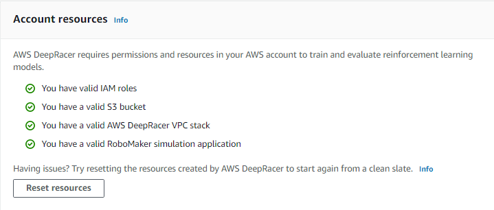
지난주 매일 1달러씩 부과 되던 NAT Gateways 서비스를 언제 세팅 했는지 몰랐었다.
여하튼 아마존 Support 서비스의 도움을 받아서 해당 서비스를 Delete 한 이후 요금은 더이상 부과 되지는 않았는데...
문제는 그걸 지우고 난 이후 Deepracer model을 생성하면 에러가 발생해서 일을 더이상 진행 할 수가 없었다.
도저히 안되서 새로운 account를 생성하고 Deepracer Model을 하나 생성했다.
그랬더니 모델과 더불어 NAT Gateways가 생성되더라.
이제 알았다. 처음 DeepRacer를 시작하기 위해 account resources를 생성할 때 이 NAT Gateway가 생성된다는 것을....
이 단계를 완료하면 NAT Gateways가 생성돼 매일 1달러씩 청구된다.
참고로 아래는 DeepRacer 모델을 하나 생성하면 청구되는 금액들이다.
* Data Transfer에서 $0.010 per GB - regional data transfer - in/out/between EC2 AZs or using elastic IPs or ELB 가 5기가가넘어서 5센트가 청구됐다.
* 그 다음 EC2에서 NAT Gateway가 생성과 연계해서 2.10 달러가 청구 됐다.
* 여기서 NAT Gateway는 매일 1달러씩 청구되게 돼 있다.
* 그 다음은 시뮬레이터 서비스인 RoboMaker 서비스에 대해 1.52달러가 청구됐고 SageMaker는 30센트가 청구됐다.
다른 서비스들은 사용하면 사용한 시간만큼만 내는데 NAT Gateway는 24시간 계속 돌아가기 때문에 매일 1불씩 내야 한다.
사용하지 않을 때 Stop 할 수도 없는 것 같다.
하루에 1달러이면 아무것도 아니라고 생각할 수 있지만... 아무것도 하지 않는데도 청구가 되니 속이 쓰렸다.
그래서 AWS Support Case를 하나 더 Raise 했다.
오늘 아침에 했는데 퇴근 할 때 쯤 답변이 오더라구.
다음은 답변 내용...
Hey there! This is Merlyn, your AWS Billing & Accounts specialist. I hope you are having a wonderful day! I understand you have some concerns about the DeepRacer pricing and you bill. Worry not as I'm here to help.
DeepRacer의 가격 책정과 청구서와 관련 우려가 있다는 것에대해 이해합니다. 걱정마세요. 제가 도와드릴테니까요.
With AWS DeepRacer console services, there are no charges for driving the AWS DeepRacer car or upfront charges. You will only pay for the AWS services you use. You will be billed separately by each of the AWS services used to provide the AWS DeepRacer console services such as creating and training your models, storing your models and logs, and evaluating them, including racing them in the virtual simulator or deploying them to their AWS DeepRacer car. You will see the bill for each service on your monthly billing statement.
AWS DeepRacer console services는 AWS DeepRacer 차량을 driving 하는데에 대한 가격 책정이나 선불로 어떠한 돈을 낼 필요가 없습니다. 당신이 AWS services를 사용한 것에 대한 요금만 지불 하시면 됩니다. AWS DeepRacer console services를 통해 사용하시는 AWS services들에 대해 각각의 사용료가 따로 청구 될 것입니다. 예를 들어 당신의 모델들을 생성하고 훈련하는 것 그리고 그 모델들이나 로그들을 저장하는 것, 그 모델들을 평가하는 작업, 가상 시뮬레이터에서 모델의 레이싱을 하거나 AWS DeepRacer car에 배치하는 일들에 대해 따로 사용료가 부과 됩니다.
Upon first use of AWS DeepRacer simulation in the AWS console, new customers will get 10 hours of Amazon SageMaker training, and 60 Simulation Unit (SU) hours for Amazon RoboMaker in the form of service credits; $6 for SageMaker, $24 for RoboMaker and $34 for NAT Gateway. The service credits are available for 30 days and applied at the end of the month. A typical AWS DeepRacer simulation uses up to six SUs per hour, thus you will be able to run a typical AWS DeepRacer simulation for up to 10 hours at no charge.
AWS console에서 AWS DeepRacer simulation을 처음 사용하는 새 고객에게는 10시간 동안 Amazon SageMaker training과 Amazon RoboMaker에 대해 60 Simulation Unit (SU) 시간에 대해 service credits이라는 형태로 무료 사용하실 수 있는 기회를 드립니다. SageMaker는 $6 , RoboMaker $24 그리고 NAT Gateway는 $34 입니다. 이 service credits은 30일간 사용 가능하고 그 달의 말에 적용됩니다. 일반적으로 AWS DeepRacer simulation 사용은 시간당 six SUs이므로 당신은 AWS DeepRacer simulation을 10시간 동안 무료로 사용하실 수 있습니다.
Please visit the link below for more pricing information:
This inquiry is a bit out of our scope. Here in the Billing and Accounts department we don’t handle technical questions. Please note that AWS unbundles technical support in order to lower the prices of the services themselves instead of billing it to all customers disregarding if they’d like to use it or not. However, if technical support is required, I would like to tell you we offer several Premium Support plans starting at just $29 a month, which enables you to speak to an engineer by email, chat, or phone depending on what support plan you choose.
당신의 요청 중 일부는 우리의 권한을 벗어나는 부분이 있습니다. 저희 Billing and Accounts department에서는 기술적인 질문은 다루지 않습니다. 저희는 모든 고객에게 비용 지불의 부담을 주지 않고 저렴한 가격을 유지하기 위해 기술 부문의 Support는 분리해서 다루고 있습니다. 만약 기술적인 support를 원하시면 월 $29 부터 시작되는 Premium Support plan 서비스들이 있습니다. 이 유료 기술 지원 서비스를 이용하시면 이메일, 채팅 그리고 전화등 여러분이 편한 방식으로 엔지니어들과 소통을 할 수 있습니다.
All Premium Support plans include direct access to Support Engineers, and these plans offer a tailored support experience that allows you to select the support level that best fits your needs. More information including pricing and how to sign up can be found here:
모든 Premium Support plan 들에는 Support Engineers과의 직접 access 권한이 포함되며 이러한 플랜들에서는 사용자의 요구 사항에 가장 적합한 서포트 레벨을 선택할 수 있는 맞춤 지원 서비스가 제공 됩니다. 가격 정책 및 가입 방법에 대한 자세한 정보는 여기를 참조하세요.
You can also search the Amazon Web Services Developer forums or post a new question. Our technical staff and the Amazon Web Services developer community participate in the forums regularly and might be able to help you. Generally, questions are responded to in about a day, though there is not a guaranteed response time.
그 외에 Amazon Web Services Developer forums에서 궁금한 내용을 검색해서 찾는 방법도 있습니다. 또한 새로운 질문을 이곳에 올릴 수도 있구요. Our technical staff와 Amazon Web Services developer community에 참여하는 개발자들로 부터 지원을 받으실 수도 있을 겁니다. 일반적으로 하루 정도 기다리면 답변을 받습니다. (응답 시간에 대한 보장은 없지만요.)
I certainly want you to have the best experience while using our services, so please feel free to let me know if you have any other concern in the meantime, it will be an honor to keep on assisting you. On behalf of Amazon Web Services, I wish you Happy Cloud Computing!
Best regards,
Merlyn N.
Amazon Web Services
==================================================================== Learn to work with the AWS Cloud. Get started with free online videos and self-paced labs at http://aws.amazon.com/training/ ====================================================================
Amazon ML supports three types of ML models: binary classification, multiclass classification, and regression. The type of model you should choose depends on the type of target that you want to predict.
Binary Classification Model
ML models for binary classification problems predict a binary outcome (one of two possible classes). To train binary classification models, Amazon ML uses the industry-standard learning algorithm known as logistic regression.
Examples of Binary Classification Problems
"Is this email spam or not spam?"
"Will the customer buy this product?"
"Is this product a book or a farm animal?"
"Is this review written by a customer or a robot?"
Multiclass Classification Model
ML models for multiclass classification problems allow you to generate predictions for multiple classes (predict one of more than two outcomes). For training multiclass models, Amazon ML uses the industry-standard learning algorithm known as multinomial logistic regression.
Examples of Multiclass Problems
"Is this product a book, movie, or clothing?"
"Is this movie a romantic comedy, documentary, or thriller?"
"Which category of products is most interesting to this customer?"
Regression Model
ML models for regression problems predict a numeric value. For training regression models, Amazon ML uses the industry-standard learning algorithm known as linear regression.
Examples of Regression Problems
"What will the temperature be in Seattle tomorrow?"
Amazon ML은 이진수 분류, 멀티클래스 분류 및 회귀라는 세 가지 유형의 ML 모델을 지원합니다. 선택해야 하는 모델 유형은 예측하려는 목표의 유형에 따라 따릅니다.
이진 분류 모델
이진 분류 문제에 대한 ML 모델은 이진 결과(가능성이 있는 두 가지 클래스 중 하나)를 예측합니다. 이진수 분류 모델을 교육하기 위해 은 '로지스틱 회귀'로 알려진 업계 표준 학습 알고리즘을 사용합니다.
이진 분류 문제의 예
"이 이메일은 스팸입니까? 스팸이 아닙니까?"
"고객이 이 제품을 구입할 것입니까?"
"이 제품은 책입니까? 아니면 가축입니까?"
"이 리뷰는 고객이 작성합니까? 로봇이 작성합니까?"
멀티클래스 분류 모델
멀티클래스 분류 문제에 대해 ML 모델을 사용하면 여러 클래스에 대한 예측을 생성할 수 있습니다(세 개 이상의 결과 중 하나를 예측). 멀티클래스 모델을 교육하기 위해 은 '다항 로지스틱 회귀'로 알려진 업계 표준 학습 알고리즘을 사용합니다.
멀티클래스 문제의 예
"이 제품은 책, 영화 또는 의류입니까?"
"이 영화는 로맨틱 코미디, 다큐멘터리 또는 스릴러입니까?"
"이 고객이 가장 관심을 갖는 제품 카테고리는 무엇입니까?"
회귀 모델
회귀 문제에 대해 ML 모델은 숫자 값을 예측합니다. 회귀 모델을 교육하기 위해 은 '선형 회귀'로 알려진 업계 표준 학습 알고리즘을 사용합니다.
회귀 문제의 예
"내일 시애틀의 기온은 어떨까요?"
"이 제품의 판매량이 얼마나 될까요?"
"이 집의 매매 가격이 얼마나 될까요?"
- Unsupervised Learning : Only data, Clustering Algorithm : Dimensionality Reduction Group words that are used in similar context or have similar meaning
- Reinforcement Learning Decision Making under uncertainty Autonomous Driving Games Reinforcement uses Reward Functions to reward correct decision and punish incorrect decision
Reinforcement learning (RL) is a machine learning technique that attempts to learn a strategy, called a policy, that optimizes an objective for an agent acting in an environment. For example, the agent might be a robot, the environment might be a maze, and the goal might be to successfully navigate the maze in the smallest amount of time. In RL, the agent takes an action, observes the state of the environment, and gets a reward based on the value of the current state of the environment. The goal is to maximize the long-term reward that the agent receives as a result of its actions. RL is well-suited for solving problems where an agent can make autonomous decisions.
RL is well-suited for solving large, complex problems. For example, supply chain management, HVAC systems, industrial robotics, game artificial intelligence, dialog systems, and autonomous vehicles. Because RL models learn by a continuous process of receiving rewards and punishments for every action taken by the agent, it is possible to train systems to make decisions under uncertainty and in dynamic environments.
Markov Decision Process (MDP)
RL is based on models called Markov Decision Processes (MDPs). An MDP consists of a series of time steps. Each time step consists of the following:
Environment
Defines the space in which the RL model operates. This can be either a real-world environment or a simulator. For example, if you train a physical autonomous vehicle on a physical road, that would be a real-world environment. If you train a computer program that models an autonomous vehicle driving on a road, that would be a simulator.
State
Specifies all information about the environment and past steps that is relevant to the future. For example, in an RL model in which a robot can move in any direction at any time step, then the position of the robot at the current time step is the state, because if we know where the robot is, it isn't necessary to know the steps it took to get there.
Action
What the agent does. For example, the robot takes a step forward.
Reward
A number that represents the value of the state that resulted from the last action that the agent took. For example, if the goal is for a robot to find treasure, the reward for finding treasure might be 5, and the reward for not finding treasure might be 0. The RL model attempts to find a strategy that optimizes the cumulative reward over the long term. This strategy is called apolicy.
Observation
Information about the state of the environment that is available to the agent at each step. This might be the entire state, or it might be just a part of the state. For example, the agent in a chess-playing model would be able to observe the entire state of the board at any step, but a robot in a maze might only be able to observe a small portion of the maze that it currently occupies.
Typically, training in RL consists of manyepisodes. An episode consists of all of the time steps in an MDP from the initial state until the environment reaches the terminal state.
Key Features of Amazon SageMaker RL
To train RL models in Amazon SageMaker RL, use the following components:
A deep learning (DL) framework. Currently, Amazon SageMaker supports RL in TensorFlow and Apache MXNet.
An RL toolkit. An RL toolkit manages the interaction between the agent and the environment, and provides a wide selection of state of the art RL algorithms. Amazon SageMaker supports the Intel Coach and Ray RLlib toolkits. For information about Intel Coach, seehttps://nervanasystems.github.io/coach/. For information about Ray RLlib, seehttps://ray.readthedocs.io/en/latest/rllib.html.
An RL environment. You can use custom environments, open-source environments, or commercial environments. For information, seeRL Environments in Amazon SageMaker.
The following diagram shows the RL components that are supported in Amazon SageMaker RL.
Amazon SageMaker RL을 사용한 강화 학습
강화 학습(RL)은 환경에서 작동하는 에이전트에 대한 목표를 최적화하는 전략(정책이라고 함)을 배우려고 시도하는 기계 학습 기법입니다. 예를 들어, 에이전트는 로봇, 환경은 미로, 목표는 최단시간 내에 미로를 성공적으로 탈출하는 것일 수 있습니다. RL에서 에이전트는 행동을 취하고, 환경의 상태를 관찰하고, 환경의 현재 상태 값에 따라 보상을 받습니다. 목표는 행동의 결과로 에이전트가 받는 장기 보상을 극대화하는 것입니다. RL은 에이전트가 자율 의사결정을 내릴 수 있는 문제를 해결하는 데 매우 적합합니다.
RL은 크고 복잡한 문제를 해결하는 데 매우 적합합니다. 예를 들어, 공급망 관리, HVAC 시스템, 산업용 로봇, 게임 인공 지능, 음성 대화 시스템 및 자율 주행 차량 등이 있습니다. RL 모델은 에이전트가 취하는 모든 행동에 대해 보상과 처벌을 받는 연속 프로세스를 통해 학습하기 때문에 동적인 환경에서 불확실성이 존재할 때 시스템이 의사를 결정하도록 훈련할 수 있습니다.
마코프 의사결정 과정(MDP)
RL은 마코프 의사결정 과정(MDP)라는 모델을 기반으로 합니다. MDP는 일련의 시간 단계로 구성됩니다. 각 시간 단계는 다음과 같은 요소로 구성됩니다.
환경
RL 모델이 작동하는 공간을 정의합니다. 이러한 공간은 실제 환경 또는 시뮬레이터일 수 있습니다. 예를 들어, 실제 도로에서 자율 주행 차량을 훈련하는 경우는 환경이 실제 환경입니다. 도로 위를 주행하는 자율 주행 차량을 모델링하는 컴퓨터 프로그램을 훈련하는 경우에는 환경이 시뮬레이터입니다.
상태
환경에 대한 모든 정보와 미래와 관련된 과거의 모든 단계를 지정합니다. 예를 들어, 로봇이 언제든지 어떤 방향으로든 이동할 수 있는 RL 모델에서는 현재 시간 단계에서 로봇의 위치가 상태입니다. 로봇 위치를 알면 해당 위치에 도착하기 위해 어떤 단계를 수행했는지 알 필요가 없기 때문입니다.
작업
작업은 에이전트가 수행합니다. 예를 들어 로봇이 앞으로 나아갑니다.
보상
에이전트가 수행한 마지막 작업의 상태 값을 나타내는 숫자입니다. 예를 들어, 목표가 로봇이 보물을 찾도록 하는 것이라면 보물을 찾은 경우 보상이 5이고, 보물을 찾지 못한 경우에는 보상이 0일 수 있습니다. RL 모델은 장기간 누적된 보상을 최적화하는 전략을 찾으려고 합니다. 이러한 전략을정책이라고 합니다.
관측치
각 단계마다 에이전트가 사용할 수 있는 환경 상태에 대한 정보입니다. 전체 상태이거나 상태의 일부분일 수 있습니다. 예를 들어, 체스 시합 모델의 에이전트는 모든 단계에서 체스판의 전체 상태를 관찰할 수 있지만 미로 속의 로봇은 현재 마주하고 있는 미로의 작은 부분 밖에 관찰할 수 없습니다.
일반적으로 RL의 훈련은 많은에피소드로 구성됩니다. 에피소드는 초기 상태에서 환경이 최종 상태에 도달할 때까지 MDP의 모든 시간 단계로 구성됩니다.
Amazon SageMaker RL의 주요 기능
Amazon SageMaker RL에서 RL 모델을 훈련하려면 다음 구성 요소를 사용합니다.
딥 러닝(DL) 프레임워크. 현재, Amazon SageMaker는 TensorFlow 및 Apache MXNet에서 RL을 지원합니다.
다음 다이어그램은 Amazon SageMaker RL에서 지원되는 RL 구성 요소를 보여 줍니다.
- refer to the picture above -
* Data types * Data in Real Life : Numeric, Text, Categorical values * Categorical : Cartesian Transformation - Combine categorical features to form new features * Text Type : NGRAM, OSB Transformation, Stemming, Lower Case * Numeric Data :
The n-gram transformation takes a text variable as input and produces strings corresponding to sliding a window of (user-configurable) n words, generating outputs in the process. For example, consider the text string "I really enjoyed reading this book".
Specifying the n-gram transformation with window size=1 simply gives you all the individual words in that string:
You can request n-grams with a size ranging from 2-10 words. N-grams with size 1 are generated implicitly for all inputs whose type is marked as text in the data schema, so you do not have to ask for them. Finally, keep in mind that n-grams are generated by breaking the input data on whitespace characters. That means that, for example, punctuation characters will be considered a part of the word tokens: generating n-grams with a window of 2 for string "red, green, blue" will yield {"red,", "green,", "blue,", "red, green", "green, blue"}. You can use the punctuation remover processor (described later in this document) to remove the punctuation symbols if this is not what you want.
To compute n-grams of window size 3 for variable var1:
"ngram(var1, 3)"
Orthogonal Sparse Bigram (OSB) Transformation
The OSB transformation is intended to aid in text string analysis and is an alternative to the bi-gram transformation (n-gram with window size 2). OSBs are generated by sliding the window of size n over the text, and outputting every pair of words that includes the first word in the window.
To build each OSB, its constituent words are joined by the "_" (underscore) character, and every skipped token is indicated by adding another underscore into the OSB. Thus, the OSB encodes not just the tokens seen within a window, but also an indication of number of tokens skipped within that same window.
To illustrate, consider the string "The quick brown fox jumps over the lazy dog", and OSBs of size 4. The six four-word windows, and the last two shorter windows from the end of the string are shown in the following example, as well OSBs generated from each:
Window, {OSBs generated}
"The quick brown fox", {The_quick, The__brown, The___fox} "quick brown fox jumps", {quick_brown, quick__fox, quick___jumps} "brown fox jumps over", {brown_fox, brown__jumps, brown___over} "fox jumps over the", {fox_jumps, fox__over, fox___the} "jumps over the lazy", {jumps_over, jumps__the, jumps___lazy} "over the lazy dog", {over_the, over__lazy, over___dog} "the lazy dog", {the_lazy, the__dog} "lazy dog", {lazy_dog}
Orthogonal sparse bigrams are an alternative for n-grams that might work better in some situations. If your data has large text fields (10 or more words), experiment to see which works better. Note that what constitutes a large text field may vary depending on the situation. However, with larger text fields, OSBs have been empirically shown to uniquely represent the text due to the specialskipsymbol (the underscore).
You can request a window size of 2 to 10 for OSB transformations on input text variables.
To compute OSBs with window size 5 for variable var1:
"osb(var1, 5)"
Lowercase Transformation
The lowercase transformation processor converts text inputs to lowercase. For example, given the input "The Quick Brown Fox Jumps Over the Lazy Dog", the processor will output "the quick brown fox jumps over the lazy dog".
To apply lowercase transformation to the variable var1:
"lowercase(var1)"
Remove Punctuation Transformation
Amazon ML implicitly splits inputs marked as text in the data schema on whitespace. Punctuation in the string ends up either adjoining word tokens, or as separate tokens entirely, depending on the whitespace surrounding it. If this is undesirable, the punctuation remover transformation may be used to remove punctuation symbols from generated features. For example, given the string "Welcome to AML - please fasten your seat-belts!", the following set of tokens is implicitly generated:
Note that only the prefix and suffix punctuation marks are removed. Punctuations that appear in the middle of a token, e.g. the hyphen in "seat-belts", are not removed.
To apply punctuation removal to the variable var1:
"no_punct(var1)"
Quantile Binning Transformation
The quantile binning processor takes two inputs, a numerical variable and a parameter calledbin number, and outputs a categorical variable. The purpose is to discover non-linearity in the variable's distribution by grouping observed values together.
In many cases, the relationship between a numeric variable and the target is not linear (the numeric variable value does not increase or decrease monotonically with the target). In such cases, it might be useful to bin the numeric feature into a categorical feature representing different ranges of the numeric feature. Each categorical feature value (bin) can then be modeled as having its own linear relationship with the target. For example, let's say you know that the continuous numeric featureaccount_ageis not linearly correlated with likelihood to purchase a book. You can bin age into categorical features that might be able to capture the relationship with the target more accurately.
The quantile binning processor can be used to instruct Amazon ML to establish n bins of equal size based on the distribution of all input values of the age variable, and then to substitute each number with a text token containing the bin. The optimum number of bins for a numeric variable is dependent on characteristics of the variable and its relationship to the target, and this is best determined through experimentation. Amazon ML suggests the optimal bin number for a numeric feature based on data statistics in theSuggested Recipe.
You can request between 5 and 1000 quantile bins to be computed for any numeric input variable.
To following example shows how to compute and use 50 bins in place of numeric variable var1:
"quantile_bin(var1, 50)"
Normalization Transformation
The normalization transformer normalizes numeric variables to have a mean of zero and variance of one. Normalization of numeric variables can help the learning process if there are very large range differences between numeric variables because variables with the highest magnitude could dominate the ML model, no matter if the feature is informative with respect to the target or not.
To apply this transformation to numeric variable var1, add this to the recipe:
normalize(var1)
This transformer can also take a user defined group of numeric variables or the pre-defined group for all numeric variables (ALL_NUMERIC) as input:
normalize(ALL_NUMERIC)
Note
It isnotmandatory to use the normalization processor for numeric variables.
Cartesian Product Transformation
The Cartesian transformation generates permutations of two or more text or categorical input variables. This transformation is used when an interaction between variables is suspected. For example, consider the bank marketing dataset that is used in Tutorial: Using Amazon ML to Predict Responses to a Marketing Offer. Using this dataset, we would like to predict whether a person would respond positively to a bank promotion, based on the economic and demographic information. We might suspect that the person's job type is somewhat important (perhaps there is a correlation between being employed in certain fields and having the money available), and the highest level of education attained is also important. We might also have a deeper intuition that there is a strong signal in the interaction of these two variables—for example, that the promotion is particularly well-suited to customers who are entrepreneurs who earned a university degree.
The Cartesian product transformation takes categorical variables or text as input, and produces new features that capture the interaction between these input variables. Specifically, for each training example, it will create a combination of features, and add them as a standalone feature. For example, let's say our simplified input rows look like this:
target, education, job
0, university.degree, technician
0, high.school, services
1, university.degree, admin
If we specify that the Cartesian transformation is to be applied to the categorical variables education and job fields, the resultant feature education_job_interaction will look like this:
target, education_job_interaction
0, university.degree_technician
0, high.school_services
1, university.degree_admin
The Cartesian transformation is even more powerful when it comes to working on sequences of tokens, as is the case when one of its arguments is a text variable that is implicitly or explicitly split into tokens. For example, consider the task of classifying a book as being a textbook or not. Intuitively, we might think that there is something about the book's title that can tell us it is a textbook (certain words might occur more frequently in textbooks' titles), and we might also think that there is something about the book's binding that is predictive (textbooks are more likely to be hardcover), but it's really the combination of some words in the title and binding that is most predictive. For a real-world example, the following table shows the results of applying the Cartesian processor to the input variables binding and title:
TextbookTitleBindingCartesian product of no_punct(Title) and Binding
n-gram 변환은 텍스트 변수를 입력으로 가져오고 (사용자가 구성 가능한) n 단어 창을 슬라이딩하는 문자열을 생성하여 해당 프로세스에서 출력을 생성합니다. 예를 들어 "I really enjoyed reading this book"이라는 텍스트 문자열을 생각해 보겠습니다.
창 크기 = 1인 n-gram 변환을 지정하면 다음과 같이 해당 문자열에 있는 모든 개별 단어가 제공됩니다.
n-gram을 2~10개 단어 범위의 크기로 요청할 수 있습니다. 크기가 1인 n-gram은 데이터 스키마에서 텍스트로 표시된 유형의 모든 입력에 대해 암시적으로 생성되므로, 사용자가 요청할 필요가 없습니다. 마지막으로, n-gram은 공백 문자에 대한 입력 데이터를 분해하여 생성된다는 것을 기억해야 합니다. 예를 들어 구두점 문자는 다음과 같이 단어 토큰의 일부로 간주됩니다. 문자열 "red, green, blue"에 대해 2개의 창으로 n-gram을 생성하면 {"red,", "green,", "blue,", "red, green", "green, blue"}로 산출됩니다. 구두점 제거 프로세서(이 문서의 뒷부분에서 설명)를 사용하여 원하지 않는 구두점을 제거할 수 있습니다.
변수 var1에 대해 창 크기가 3인 n-gram을 계산하려면:
"ngram(var1, 3)"
Orthogonal Sparse Bigram(OSB) 변환
OSB 변환은 텍스트 문자열 분석을 보조하는 목적이며 bi-gram 변환(창 크기가 2인 n-gram)을 대체하는 변환입니다. OSB는 n 단어 크기의 창을 텍스트 위로 슬라이딩하고 창의 첫 번째 단어가 포함된 모든 단어 페어를 출력하여 생성됩니다.
각 OSB를 구축하기 위해 구성 단어는 "_"(밑줄) 문자로 결합되며, 건너뛴 모든 토큰은 OSB에 또 다른 밑줄을 추가하여 표시됩니다. 따라서 OSB는 창 내에 확인되는 토큰뿐만 아니라 동일한 창 내에서 건너뛴 토큰의 수도 표시합니다.
예를 들어 "The quick brown fox jumps over the lazy dog"라는 문자열과 크기가 4인 OSB를 생각해 보겠습니다. 여섯 개의 4 단어 창 및 문자열 끝에 있는 더 짧은 길이의 마지막 창은 다음 예제에서 각 창에서 생성된 OSB와 함께 표시됩니다.
창, {생성된 OSB}
"The quick brown fox", {The_quick, The__brown, The___fox} "quick brown fox jumps", {quick_brown, quick__fox, quick___jumps} "brown fox jumps over", {brown_fox, brown__jumps, brown___over} "fox jumps over the", {fox_jumps, fox__over, fox___the} "jumps over the lazy", {jumps_over, jumps__the, jumps___lazy} "over the lazy dog", {over_the, over__lazy, over___dog} "the lazy dog", {the_lazy, the__dog} "lazy dog", {lazy_dog}
Orthogonal Sparse Bigram은 일부 상황에서 효과적으로 작용할 수 있는 n-gram의 대체 변환입니다. 데이터에 큰 텍스트 필드(10개 이상의 단어)가 있는 경우 실험을 통해 효과적인 방식을 살펴봅니다. 큰 텍스트 필드를 구성하는 내용은 상황에 따라 다를 수 있음을 참고하십시오. 그러나 큰 텍스트 필드를 사용하는 OSB는 특수건너뛰기기호(밑줄)로 인해 텍스트를 고유하게 나타내는 것으로 실증되었습니다.
입력 텍스트 변수의 OSB 변환에 대해 2~10의 창 크기를 요청할 수 있습니다.
변수 var1에 대해 창 크기가 5인 OSB를 계산하려면:
"osb(var1, 5)"
소문자 변환
소문자 변환 프로세서는 텍스트 입력을 소문자로 변환합니다. 예를 들어 프로세서는 "The Quick Brown Fox Jumps Over the Lazy Dog"라는 입력을 "the quick brown fox jumps over the lazy dog"라고 출력합니다.
변수 var1에 소문자 변환을 적용하려면:
"lowercase(var1)"
구두점 변환 제거
Amazon ML은 공백이 있는 데이터 스키마의 텍스트로 표시된 입력을 암시적으로 분리합니다. 문자열의 구두점은 주변의 공백에 따라 인접한 단어 토큰으로 끝나거나 완전히 별개의 토큰으로 끝납니다. 이것이 바람직하지 않은 경우, 생성된 특성의 구두점을 제거하는 데 구두점 제거 변환을 사용할 수 있습니다. 예를 들어 "Welcome to AML - please fasten your seat-belts!"라는 문자열이 있으면 다음과 같은 토큰 집합이 암시적으로 생성됩니다.
접두사 및 접미사 구두점만 제거됩니다. 토큰 중간에 나타나는 구두점("seat-belts"에 있는 하이픈 등)은 제거되지 않습니다.
변수 var1에 구두점 변환을 적용하려면:
"no_punct(var1)"
Quartile binning 변환
Quantile binning 프로세서는 숫자 변수 및bin number라는 파라미터의 두 가지 입력을 사용해서 카테고리 변수를 출력합니다. 그 목적은 관측된 값을 그룹화하여 변수의 배포에서 비선형성을 발견하는 것입니다.
많은 경우에 숫자 변수와 대상 간의 관계는 선형적이지 않습니다(숫자 변수 값은 대상에 따라 점차 증가하거나 감소하지 않음). 이 경우 다양한 범위의 숫자 특성을 나타내는 카테고리 특성으로 숫자 특성을 비닝하는 것이 유용할 수 있습니다. 각 카테고리 특성 값(빈)은 대상과의 선형 관계를 갖도록 모델링될 수 있습니다. 예를 들어 연속적인 숫자 특성account_age가 책을 구입할 가능성과 선형적으로 관련이 없다는 것을 알고 있다고 가정해 보겠습니다. 사용자는 대상과의 관계를 더욱 정확하게 캡처할 수 있는 카테고리 특성으로 age를 비닝할 수 있습니다.
quantile binning 프로세서는 Amazon ML이 age 변수의 모든 입력 값 배포를 기반으로 동일한 크기의 빈 n개를 설정한 다음 각 번호를 빈을 포함하는 텍스트 토큰으로 대체하도록 하는 데 사용될 수 있습니다. 숫자 변수에 대한 최적의 빈 수는 변수의 특징과 대상과의 관계에 따라 달라지며, 이는 실험을 통해 가장 효과적으로 결정됩니다. Amazon ML은제안된 레시피의 데이터 통계를 기반으로 숫자 특성에 대한 최적의 빈 수를 제시합니다.
숫자 입력 변수에 대해 5~1000개의 quantile 빈을 계산하도록 요청할 수 있습니다.
다음 예제에서는 숫자 변수 var1 대신 50개의 빈을 계산하여 사용하는 방법을 보여 줍니다.
"quantile_bin(var1, 50)"
정규화 변환
정규화 변환기는 평균 값이 0이고 분산 값이 1인 숫자 변수를 정규화합니다. 특성이 대상과 관련하여 많은 정보가 되는지 여부와 관계없이 가장 큰 크기의 변수가 ML 모델의 대부분을 차지할 수 있기 때문에, 숫자 변수의 정규화는 숫자 변수 사이에 범위 차이가 매우 큰 경우에 학습 프로세스에 도움이 될 수 있습니다.
숫자 변수 var1에 이 변환을 적용하려면 다음과 같이 레시피에 추가합니다.
normalize(var1)
이 변환기는 숫자 변수의 사용자 정의 그룹 또는 모든 숫자 변수(ALL_NUMERIC)의 사전 정의된 그룹을 입력으로 사용할 수 있습니다.
normalize(ALL_NUMERIC)
참고
숫자 변수에 정규화 프로세서를 사용하는 것은 필수가아닙니다.
데카르트 곱 변환
데카르트 변환은 두 개 이상의 텍스트 또는 카테고리 입력 변수의 순열을 생성합니다. 이 변환은 변수 간에 상호 작용이 있다고 생각될 때 사용합니다. 예를 들어 자습서: Amazon ML을 사용한 마케팅 반응 예측에서 사용되는 은행 마케팅 데이터 집합을 고려해 보겠습니다. 이 데이터 집합을 사용하여 경제 및 인구 통계 정보를 기반으로 은행 홍보에 긍정적인 반응을 보이는지 예측하려고 합니다. 해당하는 사람의 직업 유형이 상당히 중요하다고 생각할 수 있으며(특정 분야에서 근무하는 것과 사용 가능한 비용 간에 상관 관계가 있을 수 있음), 가장 높은 수준의 교육을 받은 사실도 중요하다고 간주할 수 있습니다. 또한 이 두 변수의 상호 작용에 강력한 신호가 있다는 것도 알 수 있습니다. 예를 들어 특히 학사 학위를 취득한 사업가 고객에게 홍보하는 것이 적합합니다.
데카르트 곱 변환은 카테고리 변수 또는 텍스트를 입력으로 사용하고, 이러한 입력 변수 간의 상호 작용을 캡처하는 새로운 특성을 생성합니다. 특히, 각 교육 예제에 대해 특성의 조합을 생성하고 이를 독립적인 특성으로 추가합니다. 예를 들어 다음과 같은 간소화된 입력 행이 있다고 가정하겠습니다.
target, education, job
0, university.degree, technician
0, high.school, services
1, university.degree, admin
데카르트 변환이 카테고리 변수 education 및 job 필드에 적용되도록 지정하면 결과적으로 다음과 같은 education_job_interaction 특성을 볼 수 있습니다.
target, education_job_interaction
0, university.degree_technician
0, high.school_services
1, university.degree_admin
데카르트 변환은 인수 중 하나가 암시적으로 또는 명시적으로 토큰으로 분리되는 텍스트 변수 같은 토큰 시퀀스 작업에서 더욱 강력하게 작용합니다. 예를 들어 책을 교과서로 분류할지 여부에 대한 작업을 생각해 보겠습니다. 직관적으로, 교과서라고 말할 수 있는 책의 제목에 대해 생각할 수 있으며(특정 단어는 교과서의 제목에서 더 자주 나타날 수 있음), 책의 표지에 대해 예측 가능한 점이 있다고 생각할 수도 있지만(교과서는 하드 커버가 될 가능성이 더 큼), 실제로 제목과 표지에 있는 단어의 조합이야말로 가장 예측 가능합니다. 실제 사례에서 다음 표는 데카르트 프로세서를 입력 변수 표지 및 제목에 적용한 결과를 보여 줍니다.